
This was a very fun and unique competition. It was very interesting to learn so much about a field which was very much unknown to me beforehand.
\nMy teammates solutions:
\nhttps://www.kaggle.com/competitions/ariel-data-challenge-2024/discussion/543681
\n(to be added)
First, I aggregate the signal over the spatial dimensions and use time-binning. This way, after concatenating FGS1 data and the reversed AIRS data, I get an array of size (data_size, 375, 283).
\nI calculate a weighted average of the different frequencies to reduce the signal noise with respect to the magnitude for the signal. We minimize this noise when using the inverse variances of the frequency signals as weights (after first normalizing by the magnitude of the frequency signal). This assumes only Gaussian noise, and that the noise is uncorrelated between frequencies, which is not entirely accurate. But still, I think it gives a good estimate.
Let S be the signal array for a specific sample of shape (375, 283). With the calculated variances, we can estimate the signal with the least variance relative to signal size as follows:
\nFirst we normalize each frequency by the mean signal strength:
\n$$ S'[:, i] = \\frac{S[:, i]}{Mean[S[:, i]]}$$
\n$$S_{avg} = \\sum_{i=0}^{282} \\frac{S'[:, i]}{Var[S'[:, i]]}$$
\nTo not distort this variance I don't actually just compute the variance, but rather have a method which considers the shape of the signal. Using this weighted average signal, I find the ingress and egress time by using a gaussian 1D filter over the first derivative of the signal.
\nSimilar to how it is done in public notebooks, I am searching for a polynomial that fits the curve of the incoming signal. This way I get a first estimate of the transit depth for each signal.
\nMy NN model now takes in several values as input, x_1, x_2, and x_3:
\nx_0 := The average transit depth for each signal
\nx_1[…, 0] := The unreduced differences between the polynomials and raw signals (with the transit aligned and the ingress/egress area interpolated)
\nx_1[…, 1] := The polynomials
\nx_2 := The calculated signal variances
In the network, I only use features which are invariant to scaling whenever I use non-linear activation functions. Otherwise, the model will fail because of the strong distributional shift.
\nThe model produces a global prediction for the overall transit depth. For this I again simply use the inverse invariances as weights for the different frequencies instead of a learned weighted average. I found that this generalizes a bit better.
\nMy model also produces transit depth predictions for each frequency. This is done by a 1D convolutional filter which learns a weighted average of transit depths of locally nearby frequencies. I combine the two previous predictions using another learned weighted average.
\nThe sigma prediction involves three steps:
\nI estimate the global sigma using the variance of the wavg signal and calculate a learned weighted average between this global variance and the individual frequency variances (which very slightly smoothed in frequency dimension). I average them in inverse squared space.
\nThe second way of estimating sigma is to use the profile of predicted depths as a baseline for the sigmas: depths - min(depths) (e.g. high depth predictions are more likely to be wrong). This second way gave me a very large boost in score across CV and LB (+0.03 I believe).
x_1 is normalized over the time dimension and passed into a small convolutional net to calculate small factors which are applied to the depth predictions and factors which are applied to the sigma predictions.
\nI use an LSTM which processes the min-max normalized depth and sigma predictions, adds a residual onto them, and then scales it back to restore the original min-max. This proved to be an effective way to apply deep learning without overfitting.
\nFinally, I use a custom loss function for the negative log likelihood which optimizes the predicted spectra and sigma predictions directly:
\n
My single model 2-fold CV was ~0.64 with private LB score of 0.658.
\nAnd finally, thanks to my teammates for the hard work!
", "messages": [ { "id": 3033552, "postDate": "2024-11-01T09:40:28.037Z", "content": "This was a very fun and unique competition. It was very interesting to learn so much about a field which was very much unknown to me beforehand.
\nMy teammates solutions:
\nhttps://www.kaggle.com/competitions/ariel-data-challenge-2024/discussion/543681
\n(to be added)
First, I aggregate the signal over the spatial dimensions and use time-binning. This way, after concatenating FGS1 data and the reversed AIRS data, I get an array of size (data_size, 375, 283).
\nI calculate a weighted average of the different frequencies to reduce the signal noise with respect to the magnitude for the signal. We minimize this noise when using the inverse variances of the frequency signals as weights (after first normalizing by the magnitude of the frequency signal). This assumes only Gaussian noise, and that the noise is uncorrelated between frequencies, which is not entirely accurate. But still, I think it gives a good estimate.
Let S be the signal array for a specific sample of shape (375, 283). With the calculated variances, we can estimate the signal with the least variance relative to signal size as follows:
\nFirst we normalize each frequency by the mean signal strength:
\n$$ S'[:, i] = \\frac{S[:, i]}{Mean[S[:, i]]}$$
\n$$S_{avg} = \\sum_{i=0}^{282} \\frac{S'[:, i]}{Var[S'[:, i]]}$$
\nTo not distort this variance I don't actually just compute the variance, but rather have a method which considers the shape of the signal. Using this weighted average signal, I find the ingress and egress time by using a gaussian 1D filter over the first derivative of the signal.
\nSimilar to how it is done in public notebooks, I am searching for a polynomial that fits the curve of the incoming signal. This way I get a first estimate of the transit depth for each signal.
\nMy NN model now takes in several values as input, x_1, x_2, and x_3:
\nx_0 := The average transit depth for each signal
\nx_1[…, 0] := The unreduced differences between the polynomials and raw signals (with the transit aligned and the ingress/egress area interpolated)
\nx_1[…, 1] := The polynomials
\nx_2 := The calculated signal variances
In the network, I only use features which are invariant to scaling whenever I use non-linear activation functions. Otherwise, the model will fail because of the strong distributional shift.
\nThe model produces a global prediction for the overall transit depth. For this I again simply use the inverse invariances as weights for the different frequencies instead of a learned weighted average. I found that this generalizes a bit better.
\nMy model also produces transit depth predictions for each frequency. This is done by a 1D convolutional filter which learns a weighted average of transit depths of locally nearby frequencies. I combine the two previous predictions using another learned weighted average.
\nThe sigma prediction involves three steps:
\nI estimate the global sigma using the variance of the wavg signal and calculate a learned weighted average between this global variance and the individual frequency variances (which very slightly smoothed in frequency dimension). I average them in inverse squared space.
\nThe second way of estimating sigma is to use the profile of predicted depths as a baseline for the sigmas: depths - min(depths) (e.g. high depth predictions are more likely to be wrong). This second way gave me a very large boost in score across CV and LB (+0.03 I believe).
x_1 is normalized over the time dimension and passed into a small convolutional net to calculate small factors which are applied to the depth predictions and factors which are applied to the sigma predictions.
\nI use an LSTM which processes the min-max normalized depth and sigma predictions, adds a residual onto them, and then scales it back to restore the original min-max. This proved to be an effective way to apply deep learning without overfitting.
\nFinally, I use a custom loss function for the negative log likelihood which optimizes the predicted spectra and sigma predictions directly:
\n
My single model 2-fold CV was ~0.64 with private LB score of 0.658.
\nAnd finally, thanks to my teammates for the hard work!
", "rawMarkdown": "This was a very fun and unique competition. It was very interesting to learn so much about a field which was very much unknown to me beforehand. \n\nMy teammates solutions:\nhttps://www.kaggle.com/competitions/ariel-data-challenge-2024/discussion/543681\n(to be added)\n\n\nFirst, I aggregate the signal over the spatial dimensions and use time-binning. This way, after concatenating FGS1 data and the reversed AIRS data, I get an array of size (data\\_size, 375, 283).\nI calculate a weighted average of the different frequencies to reduce the signal noise with respect to the magnitude for the signal. We minimize this noise when using the inverse variances of the frequency signals as weights (after first normalizing by the magnitude of the frequency signal). This assumes only Gaussian noise, and that the noise is uncorrelated between frequencies, which is not entirely accurate. But still, I think it gives a good estimate.\n\nLet S be the signal array for a specific sample of shape (375, 283). With the calculated variances, we can estimate the signal with the least variance relative to signal size as follows:\n\nFirst we normalize each frequency by the mean signal strength:\n\n$$ S'[:, i] = \\frac{S[:, i]}{Mean[S[:, i]]}$$\n\n$$S_{avg} = \\sum_{i=0}^{282} \\frac{S'[:, i]}{Var[S'[:, i]]}$$\n\nTo not distort this variance I don't actually just compute the variance, but rather have a method which considers the shape of the signal. Using this weighted average signal, I find the ingress and egress time by using a gaussian 1D filter over the first derivative of the signal.\n\nSimilar to how it is done in public notebooks, I am searching for a polynomial that fits the curve of the incoming signal. This way I get a first estimate of the transit depth for each signal.\n\nMy NN model now takes in several values as input, x_1, x_2, and x_3:\n**x_0** := The average transit depth for each signal\n**x_1[..., 0]** := The unreduced differences between the polynomials and raw signals (with the transit aligned and the ingress/egress area interpolated)\n**x_1[..., 1]** := The polynomials\n**x_2** := The calculated signal variances\n\nIn the network, I only use features which are invariant to scaling whenever I use non-linear activation functions. Otherwise, the model will fail because of the strong distributional shift.\n\nThe model produces a global prediction for the overall transit depth. For this I again simply use the inverse invariances as weights for the different frequencies instead of a learned weighted average. I found that this generalizes a bit better.\n\nMy model also produces transit depth predictions for each frequency. This is done by a 1D convolutional filter which learns a weighted average of transit depths of locally nearby frequencies. I combine the two previous predictions using another learned weighted average.\n\nThe sigma prediction involves three steps:\nI estimate the global sigma using the variance of the wavg signal and calculate a learned weighted average between this global variance and the individual frequency variances (which very slightly smoothed in frequency dimension). I average them in inverse squared space.\nThe second way of estimating sigma is to use the profile of predicted depths as a baseline for the sigmas: depths - min(depths) (e.g. high depth predictions are more likely to be wrong). This second way gave me a very large boost in score across CV and LB (+0.03 I believe).\n\nx_1 is normalized over the time dimension and passed into a small convolutional net to calculate small factors which are applied to the depth predictions and factors which are applied to the sigma predictions.\n\nI use an LSTM which processes the min-max normalized depth and sigma predictions, adds a residual onto them, and then scales it back to restore the original min-max. This proved to be an effective way to apply deep learning without overfitting.\n\nFinally, I use a custom loss function for the negative log likelihood which optimizes the predicted spectra and sigma predictions directly:\n\n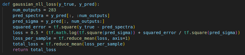\n\nMy single model 2-fold CV was ~0.64 with private LB score of 0.658.\n\nAnd finally, thanks to my teammates for the hard work!", "votes": 11 } ], "comments": [], "raw_markdown_by_id": { "3033552": "This was a very fun and unique competition. It was very interesting to learn so much about a field which was very much unknown to me beforehand. \n\nMy teammates solutions:\nhttps://www.kaggle.com/competitions/ariel-data-challenge-2024/discussion/543681\n(to be added)\n\n\nFirst, I aggregate the signal over the spatial dimensions and use time-binning. This way, after concatenating FGS1 data and the reversed AIRS data, I get an array of size (data\\_size, 375, 283).\nI calculate a weighted average of the different frequencies to reduce the signal noise with respect to the magnitude for the signal. We minimize this noise when using the inverse variances of the frequency signals as weights (after first normalizing by the magnitude of the frequency signal). This assumes only Gaussian noise, and that the noise is uncorrelated between frequencies, which is not entirely accurate. But still, I think it gives a good estimate.\n\nLet S be the signal array for a specific sample of shape (375, 283). With the calculated variances, we can estimate the signal with the least variance relative to signal size as follows:\n\nFirst we normalize each frequency by the mean signal strength:\n\n$$ S'[:, i] = \\frac{S[:, i]}{Mean[S[:, i]]}$$\n\n$$S_{avg} = \\sum_{i=0}^{282} \\frac{S'[:, i]}{Var[S'[:, i]]}$$\n\nTo not distort this variance I don't actually just compute the variance, but rather have a method which considers the shape of the signal. Using this weighted average signal, I find the ingress and egress time by using a gaussian 1D filter over the first derivative of the signal.\n\nSimilar to how it is done in public notebooks, I am searching for a polynomial that fits the curve of the incoming signal. This way I get a first estimate of the transit depth for each signal.\n\nMy NN model now takes in several values as input, x_1, x_2, and x_3:\n**x_0** := The average transit depth for each signal\n**x_1[..., 0]** := The unreduced differences between the polynomials and raw signals (with the transit aligned and the ingress/egress area interpolated)\n**x_1[..., 1]** := The polynomials\n**x_2** := The calculated signal variances\n\nIn the network, I only use features which are invariant to scaling whenever I use non-linear activation functions. Otherwise, the model will fail because of the strong distributional shift.\n\nThe model produces a global prediction for the overall transit depth. For this I again simply use the inverse invariances as weights for the different frequencies instead of a learned weighted average. I found that this generalizes a bit better.\n\nMy model also produces transit depth predictions for each frequency. This is done by a 1D convolutional filter which learns a weighted average of transit depths of locally nearby frequencies. I combine the two previous predictions using another learned weighted average.\n\nThe sigma prediction involves three steps:\nI estimate the global sigma using the variance of the wavg signal and calculate a learned weighted average between this global variance and the individual frequency variances (which very slightly smoothed in frequency dimension). I average them in inverse squared space.\nThe second way of estimating sigma is to use the profile of predicted depths as a baseline for the sigmas: depths - min(depths) (e.g. high depth predictions are more likely to be wrong). This second way gave me a very large boost in score across CV and LB (+0.03 I believe).\n\nx_1 is normalized over the time dimension and passed into a small convolutional net to calculate small factors which are applied to the depth predictions and factors which are applied to the sigma predictions.\n\nI use an LSTM which processes the min-max normalized depth and sigma predictions, adds a residual onto them, and then scales it back to restore the original min-max. This proved to be an effective way to apply deep learning without overfitting.\n\nFinally, I use a custom loss function for the negative log likelihood which optimizes the predicted spectra and sigma predictions directly:\n\n\n\nMy single model 2-fold CV was ~0.64 with private LB score of 0.658.\n\nAnd finally, thanks to my teammates for the hard work!" } }