
I'd first of all like to thank the host and the Kaggle community for this competition, it definitely was a fulfilling experience and the problem's domain is something I am particularly interested in, which made things very interesting.
\nPreprocessing
\nInitially, I did not change anything other than what was available in public notebooks, played around with time binning a little but did not get to try and use a significantly larger dataset, continued with typical 187 timepoints.
\nNoticed that removing readout noise marginally decreased RMSE of mean spectra predictions (by around 1 PPM), however I did not proceed with it.
\nI have included additional wavelengths other than the ones predicted for this challenge, around 20 to the left and to the right of the frequency band we analyzed. I got the idea that we can use these to increase the signal-to-noise ratio by binning additional wavelengths, essentially a moving window across the frequencies, an idea that I noticed many of us thought about one way or another, independently.
\nApproach
\nI have treated this challenge as 3 distinct problems, the estimation of the mean transit depth, the distribution of atmospheric features and finally, estimating uncertainty.
\nMean Transit Depth
\nIn order to calculate the mean transit depth, I first applied a Savitzky-Golay filter, with a 3rd order polynomial fit. To increase the signal-to-noise ratio, I averaged the signals from all wavelengths. After plotting a few of the resulting lightcurves, I noticed the presence of overall trends.
\nAfter calculating the transit times using derivatives, I had a polynomial fit to the out of transit period and detrended the lightcurve.
\n
Following this correction, I fit 2 more polynomials on the new, detrended lightcurve. One for the out of transit period (which essentially becomes a line, following the correction applied) and one for the in transit period. The transit depth is then given by 1 - in_transit/out_of_transit. Physically, this represents the squared ratio of the planet radius and the star radius.
\n
Repeating the derived mean for the 283 wavelengths and computing RMSE against the ground truth resulted in 97 PPM. Looking at mean depth against mean ground truth alone resulted in 43 PPM.
\nAtmospheric Features
\nI used a very simple, heavily regularized CNN architecture with 17k params:
\nKERNEL = \nPOOL = \n\n = ((a-,))\n = (, KERNEL, activation=, kernel_regularizer=(), padding=)(input_wc)\n = () (x)\n = (pool_size=POOL)(x)\n = ()(x, training = True)\n = (, KERNEL, activation=, kernel_regularizer=(), padding=)(x)\n = () (x)\n = (pool_size=POOL)(x)\n = ()(x, training = True)\n = ()(x)\n\n\n = (, activation=, kernel_regularizer=())(x)\n = ()(x, training = True)\noutput = (, activation=)()\n\nmodel = (inputs=, outputs=output)\nmodel()\nFor each planet, I had a moving window of 30 frequencies averaged and the transit depth calculated. This increased the signal-to-noise ratio and for some planets, plotting the results against the ground truth distribution showed resemblance. My bet was that there is some signal to be picked upon, and even a slight reshaping of the mean depths could significantly improve the error, granted we do not overfit to the heavy noise and niches.
\nI used the resulting depth divided by mean depth, to generate an array of coefficients centered around 1, to multiply against the mean depth computed before. So for targets, I divided each y by the y mean to get the same coefficients.
\nThe CNN resulting coefficients reduced my RMSE to 64 PPM after multiplying them against the mean depths.
\nI have implemented the CNN architecture around a week ago, and I am sure it can be improved upon and that the moving window of 30 frequencies could be optimized as well, many of the ways I tackled the problem were purely heuristic.
\nTaking the new results, I used a simple Ridge regression to try to squeeze a bit more and reduce RMSE even further, however I was very afraid of overfitting and did not have much time to play around with submissions to find an optimal tradeoff between RMSE and generalization.
\nI went ahead with an alpha that got my new RMSE to 58 PPM, even though for lower values, I could see a drop of close to 50, though my intuition tells me that's overfitting.
\nUncertainty
\nFor the sigma estimation and playing around with the GLL, I knew that in order to maximize the score, we need to predict the residuals. In a way, if you can predict the shape of the residuals, you sort of find out y_true.
\nI also believe that the uncertainty should be scaled according to the magnitude of Rp/Rs, and some planets had dramatic shifts there (+- 50%), so the tradeoff between accuracy and overshooting/undershooting was one of the harder parts of this competition.
\nI tried multiple ways, including having another linear model predict residuals, resulting in CV scores as high as 0.66, yet nothing translated to the LB. I did not play around with only doing this for the known stars, I believe this could somehow translate more to the LB, while using a more conservative sigma for the unknown stars.
\nIn the end, through trial and error, I found three approaches which worked very well for the local score: the standard deviation of the prediction, the median of the residuals and the standard deviation of the residuals.
\nMy highest scoring result is using a simple, conservative 2 standard deviations of the predictions for each planet.
\nI believe that fiddling around with the distribution of sigma across the 283 wavelengths could definitely be an approachable way to improve the score (against predicting the same uncertainty across all points for the planet), but I lacked the time to dive deep into this particular part of the problem. This is obvious when looking at some particular plots, where a static sigma is clearly not optimal.
\n
Closing thoughts
\nThis has been my second live competition on Kaggle and another great learning experience. I am continuously in awe reading the discussion boards and the amount of knowledge sharing people are doing. I want to thank you all for the opportunity to do this and improve my understanding of Machine Learning.
\nI am definitely looking forward to the Ariel Data Challenge for 2025 and plan on participating again.
", "messages": [ { "id": 3033639, "postDate": "2024-11-01T11:33:42.150Z", "content": "I'd first of all like to thank the host and the Kaggle community for this competition, it definitely was a fulfilling experience and the problem's domain is something I am particularly interested in, which made things very interesting.
\nPreprocessing
\nInitially, I did not change anything other than what was available in public notebooks, played around with time binning a little but did not get to try and use a significantly larger dataset, continued with typical 187 timepoints.
\nNoticed that removing readout noise marginally decreased RMSE of mean spectra predictions (by around 1 PPM), however I did not proceed with it.
\nI have included additional wavelengths other than the ones predicted for this challenge, around 20 to the left and to the right of the frequency band we analyzed. I got the idea that we can use these to increase the signal-to-noise ratio by binning additional wavelengths, essentially a moving window across the frequencies, an idea that I noticed many of us thought about one way or another, independently.
\nApproach
\nI have treated this challenge as 3 distinct problems, the estimation of the mean transit depth, the distribution of atmospheric features and finally, estimating uncertainty.
\nMean Transit Depth
\nIn order to calculate the mean transit depth, I first applied a Savitzky-Golay filter, with a 3rd order polynomial fit. To increase the signal-to-noise ratio, I averaged the signals from all wavelengths. After plotting a few of the resulting lightcurves, I noticed the presence of overall trends.
\nAfter calculating the transit times using derivatives, I had a polynomial fit to the out of transit period and detrended the lightcurve.
\n
Following this correction, I fit 2 more polynomials on the new, detrended lightcurve. One for the out of transit period (which essentially becomes a line, following the correction applied) and one for the in transit period. The transit depth is then given by 1 - in_transit/out_of_transit. Physically, this represents the squared ratio of the planet radius and the star radius.
\n
Repeating the derived mean for the 283 wavelengths and computing RMSE against the ground truth resulted in 97 PPM. Looking at mean depth against mean ground truth alone resulted in 43 PPM.
\nAtmospheric Features
\nI used a very simple, heavily regularized CNN architecture with 17k params:
\nKERNEL = \nPOOL = \n\n = ((a-,))\n = (, KERNEL, activation=, kernel_regularizer=(), padding=)(input_wc)\n = () (x)\n = (pool_size=POOL)(x)\n = ()(x, training = True)\n = (, KERNEL, activation=, kernel_regularizer=(), padding=)(x)\n = () (x)\n = (pool_size=POOL)(x)\n = ()(x, training = True)\n = ()(x)\n\n\n = (, activation=, kernel_regularizer=())(x)\n = ()(x, training = True)\noutput = (, activation=)()\n\nmodel = (inputs=, outputs=output)\nmodel()\nFor each planet, I had a moving window of 30 frequencies averaged and the transit depth calculated. This increased the signal-to-noise ratio and for some planets, plotting the results against the ground truth distribution showed resemblance. My bet was that there is some signal to be picked upon, and even a slight reshaping of the mean depths could significantly improve the error, granted we do not overfit to the heavy noise and niches.
\nI used the resulting depth divided by mean depth, to generate an array of coefficients centered around 1, to multiply against the mean depth computed before. So for targets, I divided each y by the y mean to get the same coefficients.
\nThe CNN resulting coefficients reduced my RMSE to 64 PPM after multiplying them against the mean depths.
\nI have implemented the CNN architecture around a week ago, and I am sure it can be improved upon and that the moving window of 30 frequencies could be optimized as well, many of the ways I tackled the problem were purely heuristic.
\nTaking the new results, I used a simple Ridge regression to try to squeeze a bit more and reduce RMSE even further, however I was very afraid of overfitting and did not have much time to play around with submissions to find an optimal tradeoff between RMSE and generalization.
\nI went ahead with an alpha that got my new RMSE to 58 PPM, even though for lower values, I could see a drop of close to 50, though my intuition tells me that's overfitting.
\nUncertainty
\nFor the sigma estimation and playing around with the GLL, I knew that in order to maximize the score, we need to predict the residuals. In a way, if you can predict the shape of the residuals, you sort of find out y_true.
\nI also believe that the uncertainty should be scaled according to the magnitude of Rp/Rs, and some planets had dramatic shifts there (+- 50%), so the tradeoff between accuracy and overshooting/undershooting was one of the harder parts of this competition.
\nI tried multiple ways, including having another linear model predict residuals, resulting in CV scores as high as 0.66, yet nothing translated to the LB. I did not play around with only doing this for the known stars, I believe this could somehow translate more to the LB, while using a more conservative sigma for the unknown stars.
\nIn the end, through trial and error, I found three approaches which worked very well for the local score: the standard deviation of the prediction, the median of the residuals and the standard deviation of the residuals.
\nMy highest scoring result is using a simple, conservative 2 standard deviations of the predictions for each planet.
\nI believe that fiddling around with the distribution of sigma across the 283 wavelengths could definitely be an approachable way to improve the score (against predicting the same uncertainty across all points for the planet), but I lacked the time to dive deep into this particular part of the problem. This is obvious when looking at some particular plots, where a static sigma is clearly not optimal.
\n
Closing thoughts
\nThis has been my second live competition on Kaggle and another great learning experience. I am continuously in awe reading the discussion boards and the amount of knowledge sharing people are doing. I want to thank you all for the opportunity to do this and improve my understanding of Machine Learning.
\nI am definitely looking forward to the Ariel Data Challenge for 2025 and plan on participating again.
", "rawMarkdown": "I'd first of all like to thank the host and the Kaggle community for this competition, it definitely was a fulfilling experience and the problem's domain is something I am particularly interested in, which made things very interesting.\n\n\n**Preprocessing**\n\nInitially, I did not change anything other than what was available in public notebooks, played around with time binning a little but did not get to try and use a significantly larger dataset, continued with typical 187 timepoints.\n\nNoticed that removing readout noise marginally decreased RMSE of mean spectra predictions (by around 1 PPM), however I did not proceed with it. \n\nI have included additional wavelengths other than the ones predicted for this challenge, around 20 to the left and to the right of the frequency band we analyzed. I got the idea that we can use these to increase the signal-to-noise ratio by binning additional wavelengths, essentially a moving window across the frequencies, an idea that I noticed many of us thought about one way or another, independently.\n\n**Approach**\n\nI have treated this challenge as 3 distinct problems, the estimation of the *mean transit depth*, the distribution of *atmospheric features* and finally, estimating *uncertainty*. \n\n**Mean Transit Depth**\n\nIn order to calculate the mean transit depth, I first applied a Savitzky-Golay filter, with a 3rd order polynomial fit. To increase the signal-to-noise ratio, I averaged the signals from all wavelengths. After plotting a few of the resulting lightcurves, I noticed the presence of overall trends.\n\nAfter calculating the transit times using derivatives, I had a polynomial fit to the out of transit period and detrended the lightcurve.\n\n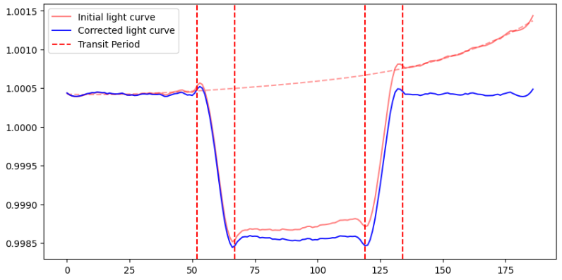\n\nFollowing this correction, I fit 2 more polynomials on the new, detrended lightcurve. One for the out of transit period (which essentially becomes a line, following the correction applied) and one for the in transit period. The transit depth is then given by 1 - in_transit/out_of_transit. Physically, this represents the squared ratio of the planet radius and the star radius.\n\n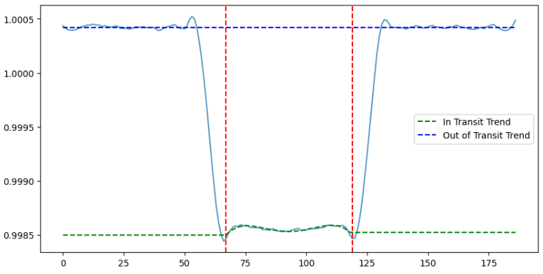\n\nRepeating the derived mean for the 283 wavelengths and computing RMSE against the ground truth resulted in 97 PPM. Looking at mean depth against mean ground truth alone resulted in 43 PPM.\n\n**Atmospheric Features**\n\nI used a very simple, heavily regularized CNN architecture with 17k params:\n```\nKERNEL = 11\nPOOL = 2\n\ninput = Input((a-1,1))\nx = Conv1D(8, KERNEL, activation='relu', kernel_regularizer=l2(0.001), padding='same')(input_wc)\nx = BatchNormalization() (x)\nx = MaxPooling1D(pool_size=POOL)(x)\nx = Dropout(0.5)(x, training = True)\nx = Conv1D(16, KERNEL, activation='relu', kernel_regularizer=l2(0.001), padding='same')(x)\nx = BatchNormalization() (x)\nx = MaxPooling1D(pool_size=POOL)(x)\nx = Dropout(0.5)(x, training = True)\nx = Flatten()(x)\n\n\nx = Dense(32, activation='relu', kernel_regularizer=l2(0.001))(x)\nx = Dropout(0.5)(x, training = True)\noutput = Dense(283, activation='linear')(x)\n\nmodel = Model(inputs=input, outputs=output)\nmodel.summary()\n```\n\nFor each planet, I had a moving window of 30 frequencies averaged and the transit depth calculated. This increased the signal-to-noise ratio and for some planets, plotting the results against the ground truth distribution showed resemblance. My bet was that there is some signal to be picked upon, and even a slight reshaping of the mean depths could significantly improve the error, granted we do not overfit to the heavy noise and niches.\n\nI used the resulting depth divided by mean depth, to generate an array of coefficients centered around 1, to multiply against the mean depth computed before. So for targets, I divided each y by the y mean to get the same coefficients.\n\nThe CNN resulting coefficients reduced my RMSE to 64 PPM after multiplying them against the mean depths.\n\nI have implemented the CNN architecture around a week ago, and I am sure it can be improved upon and that the moving window of 30 frequencies could be optimized as well, many of the ways I tackled the problem were purely heuristic.\n\nTaking the new results, I used a simple Ridge regression to try to squeeze a bit more and reduce RMSE even further, however I was very afraid of overfitting and did not have much time to play around with submissions to find an optimal tradeoff between RMSE and generalization. \n\nI went ahead with an alpha that got my new RMSE to 58 PPM, even though for lower values, I could see a drop of close to 50, though my intuition tells me that's overfitting.\n\n**Uncertainty**\n\nFor the sigma estimation and playing around with the GLL, I knew that in order to maximize the score, we need to predict the residuals. In a way, if you can predict the shape of the residuals, you sort of find out y_true.\n\nI also believe that the uncertainty should be scaled according to the magnitude of Rp/Rs, and some planets had dramatic shifts there (+- 50%), so the tradeoff between accuracy and overshooting/undershooting was one of the harder parts of this competition.\n\nI tried multiple ways, including having another linear model predict residuals, resulting in CV scores as high as 0.66, yet nothing translated to the LB. I did not play around with only doing this for the known stars, I believe this could somehow translate more to the LB, while using a more conservative sigma for the unknown stars.\n\nIn the end, through trial and error, I found three approaches which worked very well for the local score: the standard deviation of the prediction, the median of the residuals and the standard deviation of the residuals.\n\nMy highest scoring result is using a simple, conservative 2 standard deviations of the predictions for each planet.\n\nI believe that fiddling around with the distribution of sigma across the 283 wavelengths could definitely be an approachable way to improve the score (against predicting the same uncertainty across all points for the planet), but I lacked the time to dive deep into this particular part of the problem. This is obvious when looking at some particular plots, where a static sigma is clearly not optimal.\n\n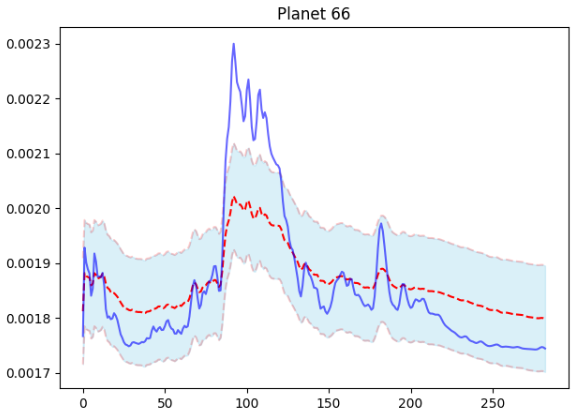\n\n**Closing thoughts**\n\nThis has been my second live competition on Kaggle and another great learning experience. I am continuously in awe reading the discussion boards and the amount of knowledge sharing people are doing. I want to thank you all for the opportunity to do this and improve my understanding of Machine Learning.\n\nI am definitely looking forward to the Ariel Data Challenge for 2025 and plan on participating again.", "votes": 7 } ], "comments": [], "raw_markdown_by_id": { "3033639": "I'd first of all like to thank the host and the Kaggle community for this competition, it definitely was a fulfilling experience and the problem's domain is something I am particularly interested in, which made things very interesting.\n\n\n**Preprocessing**\n\nInitially, I did not change anything other than what was available in public notebooks, played around with time binning a little but did not get to try and use a significantly larger dataset, continued with typical 187 timepoints.\n\nNoticed that removing readout noise marginally decreased RMSE of mean spectra predictions (by around 1 PPM), however I did not proceed with it. \n\nI have included additional wavelengths other than the ones predicted for this challenge, around 20 to the left and to the right of the frequency band we analyzed. I got the idea that we can use these to increase the signal-to-noise ratio by binning additional wavelengths, essentially a moving window across the frequencies, an idea that I noticed many of us thought about one way or another, independently.\n\n**Approach**\n\nI have treated this challenge as 3 distinct problems, the estimation of the *mean transit depth*, the distribution of *atmospheric features* and finally, estimating *uncertainty*. \n\n**Mean Transit Depth**\n\nIn order to calculate the mean transit depth, I first applied a Savitzky-Golay filter, with a 3rd order polynomial fit. To increase the signal-to-noise ratio, I averaged the signals from all wavelengths. After plotting a few of the resulting lightcurves, I noticed the presence of overall trends.\n\nAfter calculating the transit times using derivatives, I had a polynomial fit to the out of transit period and detrended the lightcurve.\n\n\n\nFollowing this correction, I fit 2 more polynomials on the new, detrended lightcurve. One for the out of transit period (which essentially becomes a line, following the correction applied) and one for the in transit period. The transit depth is then given by 1 - in_transit/out_of_transit. Physically, this represents the squared ratio of the planet radius and the star radius.\n\n\n\nRepeating the derived mean for the 283 wavelengths and computing RMSE against the ground truth resulted in 97 PPM. Looking at mean depth against mean ground truth alone resulted in 43 PPM.\n\n**Atmospheric Features**\n\nI used a very simple, heavily regularized CNN architecture with 17k params:\n```\nKERNEL = 11\nPOOL = 2\n\ninput = Input((a-1,1))\nx = Conv1D(8, KERNEL, activation='relu', kernel_regularizer=l2(0.001), padding='same')(input_wc)\nx = BatchNormalization() (x)\nx = MaxPooling1D(pool_size=POOL)(x)\nx = Dropout(0.5)(x, training = True)\nx = Conv1D(16, KERNEL, activation='relu', kernel_regularizer=l2(0.001), padding='same')(x)\nx = BatchNormalization() (x)\nx = MaxPooling1D(pool_size=POOL)(x)\nx = Dropout(0.5)(x, training = True)\nx = Flatten()(x)\n\n\nx = Dense(32, activation='relu', kernel_regularizer=l2(0.001))(x)\nx = Dropout(0.5)(x, training = True)\noutput = Dense(283, activation='linear')(x)\n\nmodel = Model(inputs=input, outputs=output)\nmodel.summary()\n```\n\nFor each planet, I had a moving window of 30 frequencies averaged and the transit depth calculated. This increased the signal-to-noise ratio and for some planets, plotting the results against the ground truth distribution showed resemblance. My bet was that there is some signal to be picked upon, and even a slight reshaping of the mean depths could significantly improve the error, granted we do not overfit to the heavy noise and niches.\n\nI used the resulting depth divided by mean depth, to generate an array of coefficients centered around 1, to multiply against the mean depth computed before. So for targets, I divided each y by the y mean to get the same coefficients.\n\nThe CNN resulting coefficients reduced my RMSE to 64 PPM after multiplying them against the mean depths.\n\nI have implemented the CNN architecture around a week ago, and I am sure it can be improved upon and that the moving window of 30 frequencies could be optimized as well, many of the ways I tackled the problem were purely heuristic.\n\nTaking the new results, I used a simple Ridge regression to try to squeeze a bit more and reduce RMSE even further, however I was very afraid of overfitting and did not have much time to play around with submissions to find an optimal tradeoff between RMSE and generalization. \n\nI went ahead with an alpha that got my new RMSE to 58 PPM, even though for lower values, I could see a drop of close to 50, though my intuition tells me that's overfitting.\n\n**Uncertainty**\n\nFor the sigma estimation and playing around with the GLL, I knew that in order to maximize the score, we need to predict the residuals. In a way, if you can predict the shape of the residuals, you sort of find out y_true.\n\nI also believe that the uncertainty should be scaled according to the magnitude of Rp/Rs, and some planets had dramatic shifts there (+- 50%), so the tradeoff between accuracy and overshooting/undershooting was one of the harder parts of this competition.\n\nI tried multiple ways, including having another linear model predict residuals, resulting in CV scores as high as 0.66, yet nothing translated to the LB. I did not play around with only doing this for the known stars, I believe this could somehow translate more to the LB, while using a more conservative sigma for the unknown stars.\n\nIn the end, through trial and error, I found three approaches which worked very well for the local score: the standard deviation of the prediction, the median of the residuals and the standard deviation of the residuals.\n\nMy highest scoring result is using a simple, conservative 2 standard deviations of the predictions for each planet.\n\nI believe that fiddling around with the distribution of sigma across the 283 wavelengths could definitely be an approachable way to improve the score (against predicting the same uncertainty across all points for the planet), but I lacked the time to dive deep into this particular part of the problem. This is obvious when looking at some particular plots, where a static sigma is clearly not optimal.\n\n\n\n**Closing thoughts**\n\nThis has been my second live competition on Kaggle and another great learning experience. I am continuously in awe reading the discussion boards and the amount of knowledge sharing people are doing. I want to thank you all for the opportunity to do this and improve my understanding of Machine Learning.\n\nI am definitely looking forward to the Ariel Data Challenge for 2025 and plan on participating again." } }