
Link to submission code: https://www.kaggle.com/code/jeroencottaar/ariel-2nd-place-submission-notebook
\nLink to visualization code: https://www.kaggle.com/code/jeroencottaar/ariel-2nd-place-visualization-notebook
Looking for opportunities and guidance: the Bayesian Inference approach I describe below is good for much more than competitions - it's applicable to many real-world problems, and is underused in our deep-learning-oriented times. I believe I can meaningfully impact our world with my knowledge of these techniques, but am currently struggling to find the right path in my career to achieve this. If you have insights on how to make a more significant impact with Bayesian methods, I’d be grateful for any guidance, perhaps in a mentorship capacity.
\nTransit analysis is the most common method for detecting and studying exoplanets. A transit occurs when a planet crosses in front of its star relative to Earth, obscuring part of the starlight. By observing how much the light is reduced (the transit depth) as a function of wavelength, we can learn the properties of the planet. But with a tiny planet passing in front of a huge star, this problem has a very low signal to noise ratio. The challenge to us: find the transit depth, including confidence intervals, from synthetic raw spectroscopic signals as the Ariel satellite might see them in the future (For a more extensive overview, see https://www.kaggle.com/competitions/ariel-data-challenge-2024/overview).
\n
My solution to this challenge is built on the related concepts of Bayesian Inference and Gaussian Processes.
\nBayesian Inference (BI) is a powerful statistical approach, based around defining a prior (a statistical belief about reality) and observations (some form of new information). Using Bayes' law, we then combined these to find the posterior (an updated belief about reality). In our case, this means:
\nTo me, the most attractive element of BI is how it lets us split our physical thinking from our solver. All our domain knowledge goes into defining the prior, where we can consider one physical element at a time; doing the actual Bayesian Inference to find the posterior is then 'just math'. Not necessarily easy math - but it's entirely separate from our domain knowledge.
\nThe figure below shows how one example transit is split in the posterior:
\n
Several of our prior elements are smooth functions; for example, transit depth is a function of wavelength, drift is a function of wavelength and time, etc. This means that we need to describe a distribution of functions in the prior. Gaussian Processes (GPs) are a natural way to do this. GPs are non-parametric methods, meaning they do not rely on a fixed set of basis functions. Instead, they allow any function, but assign different probabilities to different functions. For example, a low-frequent drift is more likely than a high-frequent one. An excellent starting point to learn GPs is https://arxiv.org/abs/2009.10862
\nIn my post here, I'll mainly focus on providing the details of the model, which in the BI framework just means describing the prior. At the end I'll cover some odds and ends (preprocessing and how we actually do the BI math).
\nIn this section I'll provide some visual breakdowns, an overview of the various elements, and some notes. You will see references to separate sensors (AIRS and FGS), but I don't really discuss my use of these sensors; The AIRS is the main sensor (the spectroscope). This section assumes familiarity with GPs, but hopefully you can get the gist of it in any case. If you want to know all the details, you'll have to go into the code (ariel_gp.py).
\n
\n
| Prior element | \nDescription | \nTuning and hyperparameters | \nDegrees of freedom | \n
|---|---|---|---|
| Noise | \nUncorrelated Gaussian per time and wavelength | \nStandard deviations found in preprocessing | \n114340 | \n
| Star spectrum | \nUncorrelated value per wavelength | \nNot regularized (infinite sigma) | \n283 | \n
| Drift: 1D | \n2x GP over time, 1 for AIRS and 1 for FGS | \nTuned on training set | \n816 | \n
| Drift: 2D | \nGP over time and wavelength | \nTuned on training set | \n113928 -> 800 with KISS-GP | \n
| Transit window | \nFixed function, ingress/egress time and width are fit | \nFixed function is found on training set | \n3 | \n
| Transit depth: mean | \nSingle value | \nNot regularized | \n1 | \n
| Transit depth: variation FGS | \nSingle Gaussian value | \nStandard deviation found on training set | \n1 | \n
| Transit depth: variation AIRS | \nGP over wavelength | \nTuned on training set | \n282 | \n
| Transit depth: PCA | \nFixed basis functions obtained from PCA analysis | \nPCA shapes found from an initial rough fit on test data | \n1 | \n
Notes on the details:
\n(EDIT: I since learned from @cnumber that this is due to the fact that I missed a constant background signal; if you turn on include_later_optimization in the code this will be corrected for, and both of these fudge values are disabled)
\nMy general preprocessing flow is as follows (details in ariel_support.py):
\nI actually have a more involved alternative that includes jitter correction and weighted column summation (to reduce the overall noise). I think these things are needed for optimal performance, but I didn't see enough gain to justify the additional complexity (though I've now seen that I actually some unselected first place submissions with this alternative flow…)
\nAs described in the introduction, actually finding the posterior in BI is 'just math' - there's no domain knowledge involved anymore. But we do of course have to implement the math as well. Some notes on this:
\nBy applying Bayesian Inference, we can disentangle the complexity of our model. We can consider each of our physical contributors (noise, drift, transit, etc.) on their own, and separate all that from the actual math of the solver. This leads to a powerful and flexible model - for example, if we need to add additional physics like limb darkening, we only touch one of the elements of the model. Finally, it also provides accurate error estimates - including full covariance matrices per planet, which will be critical for accurate further modeling. I am convinced Bayesian Inference is the way to go for the Ariel project.
\nIf you have any ideas on how I can increase my impact using these Bayesian methods, or simply recognize the challenge, please get in touch!
", "messages": [ { "id": 3034133, "postDate": "2024-11-01T19:50:00.347Z", "content": "Link to submission code: https://www.kaggle.com/code/jeroencottaar/ariel-2nd-place-submission-notebook
\nLink to visualization code: https://www.kaggle.com/code/jeroencottaar/ariel-2nd-place-visualization-notebook
Looking for opportunities and guidance: the Bayesian Inference approach I describe below is good for much more than competitions - it's applicable to many real-world problems, and is underused in our deep-learning-oriented times. I believe I can meaningfully impact our world with my knowledge of these techniques, but am currently struggling to find the right path in my career to achieve this. If you have insights on how to make a more significant impact with Bayesian methods, I’d be grateful for any guidance, perhaps in a mentorship capacity.
\nTransit analysis is the most common method for detecting and studying exoplanets. A transit occurs when a planet crosses in front of its star relative to Earth, obscuring part of the starlight. By observing how much the light is reduced (the transit depth) as a function of wavelength, we can learn the properties of the planet. But with a tiny planet passing in front of a huge star, this problem has a very low signal to noise ratio. The challenge to us: find the transit depth, including confidence intervals, from synthetic raw spectroscopic signals as the Ariel satellite might see them in the future (For a more extensive overview, see https://www.kaggle.com/competitions/ariel-data-challenge-2024/overview).
\n
My solution to this challenge is built on the related concepts of Bayesian Inference and Gaussian Processes.
\nBayesian Inference (BI) is a powerful statistical approach, based around defining a prior (a statistical belief about reality) and observations (some form of new information). Using Bayes' law, we then combined these to find the posterior (an updated belief about reality). In our case, this means:
\nTo me, the most attractive element of BI is how it lets us split our physical thinking from our solver. All our domain knowledge goes into defining the prior, where we can consider one physical element at a time; doing the actual Bayesian Inference to find the posterior is then 'just math'. Not necessarily easy math - but it's entirely separate from our domain knowledge.
\nThe figure below shows how one example transit is split in the posterior:
\n
Several of our prior elements are smooth functions; for example, transit depth is a function of wavelength, drift is a function of wavelength and time, etc. This means that we need to describe a distribution of functions in the prior. Gaussian Processes (GPs) are a natural way to do this. GPs are non-parametric methods, meaning they do not rely on a fixed set of basis functions. Instead, they allow any function, but assign different probabilities to different functions. For example, a low-frequent drift is more likely than a high-frequent one. An excellent starting point to learn GPs is https://arxiv.org/abs/2009.10862
\nIn my post here, I'll mainly focus on providing the details of the model, which in the BI framework just means describing the prior. At the end I'll cover some odds and ends (preprocessing and how we actually do the BI math).
\nIn this section I'll provide some visual breakdowns, an overview of the various elements, and some notes. You will see references to separate sensors (AIRS and FGS), but I don't really discuss my use of these sensors; The AIRS is the main sensor (the spectroscope). This section assumes familiarity with GPs, but hopefully you can get the gist of it in any case. If you want to know all the details, you'll have to go into the code (ariel_gp.py).
\n
\n
| Prior element | \nDescription | \nTuning and hyperparameters | \nDegrees of freedom | \n
|---|---|---|---|
| Noise | \nUncorrelated Gaussian per time and wavelength | \nStandard deviations found in preprocessing | \n114340 | \n
| Star spectrum | \nUncorrelated value per wavelength | \nNot regularized (infinite sigma) | \n283 | \n
| Drift: 1D | \n2x GP over time, 1 for AIRS and 1 for FGS | \nTuned on training set | \n816 | \n
| Drift: 2D | \nGP over time and wavelength | \nTuned on training set | \n113928 -> 800 with KISS-GP | \n
| Transit window | \nFixed function, ingress/egress time and width are fit | \nFixed function is found on training set | \n3 | \n
| Transit depth: mean | \nSingle value | \nNot regularized | \n1 | \n
| Transit depth: variation FGS | \nSingle Gaussian value | \nStandard deviation found on training set | \n1 | \n
| Transit depth: variation AIRS | \nGP over wavelength | \nTuned on training set | \n282 | \n
| Transit depth: PCA | \nFixed basis functions obtained from PCA analysis | \nPCA shapes found from an initial rough fit on test data | \n1 | \n
Notes on the details:
\n(EDIT: I since learned from @cnumber that this is due to the fact that I missed a constant background signal; if you turn on include_later_optimization in the code this will be corrected for, and both of these fudge values are disabled)
\nMy general preprocessing flow is as follows (details in ariel_support.py):
\nI actually have a more involved alternative that includes jitter correction and weighted column summation (to reduce the overall noise). I think these things are needed for optimal performance, but I didn't see enough gain to justify the additional complexity (though I've now seen that I actually some unselected first place submissions with this alternative flow…)
\nAs described in the introduction, actually finding the posterior in BI is 'just math' - there's no domain knowledge involved anymore. But we do of course have to implement the math as well. Some notes on this:
\nBy applying Bayesian Inference, we can disentangle the complexity of our model. We can consider each of our physical contributors (noise, drift, transit, etc.) on their own, and separate all that from the actual math of the solver. This leads to a powerful and flexible model - for example, if we need to add additional physics like limb darkening, we only touch one of the elements of the model. Finally, it also provides accurate error estimates - including full covariance matrices per planet, which will be critical for accurate further modeling. I am convinced Bayesian Inference is the way to go for the Ariel project.
\nIf you have any ideas on how I can increase my impact using these Bayesian methods, or simply recognize the challenge, please get in touch!
", "rawMarkdown": "**Link to submission code**: https://www.kaggle.com/code/jeroencottaar/ariel-2nd-place-submission-notebook \n**Link to visualization code**: https://www.kaggle.com/code/jeroencottaar/ariel-2nd-place-visualization-notebook\n\n**Looking for opportunities and guidance**: the Bayesian Inference approach I describe below is good for much more than competitions - it's applicable to many real-world problems, and is underused in our deep-learning-oriented times. I believe I can meaningfully impact our world with my knowledge of these techniques, but am currently struggling to find the right path in my career to achieve this. If you have insights on how to make a more significant impact with Bayesian methods, I’d be grateful for any guidance, perhaps in a mentorship capacity.\n\n## Introduction\n\nTransit analysis is the most common method for detecting and studying exoplanets. A transit occurs when a planet crosses in front of its star relative to Earth, obscuring part of the starlight. By observing how much the light is reduced (the transit depth) as a function of wavelength, we can learn the properties of the planet. But with a tiny planet passing in front of a huge star, this problem has a very low signal to noise ratio. The challenge to us: find the transit depth, including confidence intervals, from synthetic raw spectroscopic signals as the Ariel satellite might see them in the future (For a more extensive overview, see https://www.kaggle.com/competitions/ariel-data-challenge-2024/overview).\n\n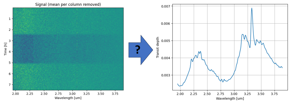\n\nMy solution to this challenge is built on the related concepts of **Bayesian Inference** and **Gaussian Processes**.\n\n**Bayesian Inference** (BI) is a powerful statistical approach, based around defining a *prior* (a statistical belief about reality) and *observations* (some form of new information). Using Bayes' law, we then combined these to find the *posterior* (an updated belief about reality). In our case, this means:\n- **Prior**: a description of the physics that affect the final measured signal, describing for example detector noise, drift, and the transit behavior (including the transit depth itself) as formal distributions.\n- **Observations**: the provided measurements.\n- **Posterior**: a breakdown of the observations into the various elements defined in the prior (see figure below). From this we can simply read out the desired transit depth. Importantly, the posterior is not just a single point, it's a distribution. By taking samples from this distribution we can find the required confidence intervals (and even full covariance matrices, although that is not asked of us here).\n\nTo me, the most attractive element of BI is how it lets us split our physical thinking from our solver. All our domain knowledge goes into defining the prior, where we can consider one physical element at a time; doing the actual Bayesian Inference to find the posterior is then 'just math'. Not necessarily easy math - but it's entirely separate from our domain knowledge. \n\nThe figure below shows how one example transit is split in the posterior:\n\n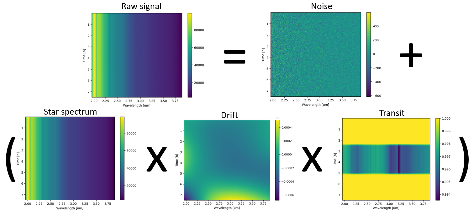\n\nSeveral of our prior elements are smooth functions; for example, transit depth is a function of wavelength, drift is a function of wavelength and time, etc. This means that we need to describe a distribution of functions in the prior. **Gaussian Processes** (GPs) are a natural way to do this. GPs are non-parametric methods, meaning they do not rely on a fixed set of basis functions. Instead, they allow any function, but assign different probabilities to different functions. For example, a low-frequent drift is more likely than a high-frequent one. An excellent starting point to learn GPs is https://arxiv.org/abs/2009.10862\n\nIn my post here, I'll mainly focus on providing the details of the model, which in the BI framework just means describing the prior. At the end I'll cover some odds and ends (preprocessing and how we actually do the BI math).\n## Prior definition\n\nIn this section I'll provide some visual breakdowns, an overview of the various elements, and some notes. You will see references to separate sensors (AIRS and FGS), but I don't really discuss my use of these sensors; The AIRS is the main sensor (the spectroscope). This section assumes familiarity with GPs, but hopefully you can get the gist of it in any case. If you want to know all the details, you'll have to go into the code (ariel_gp.py). \n\n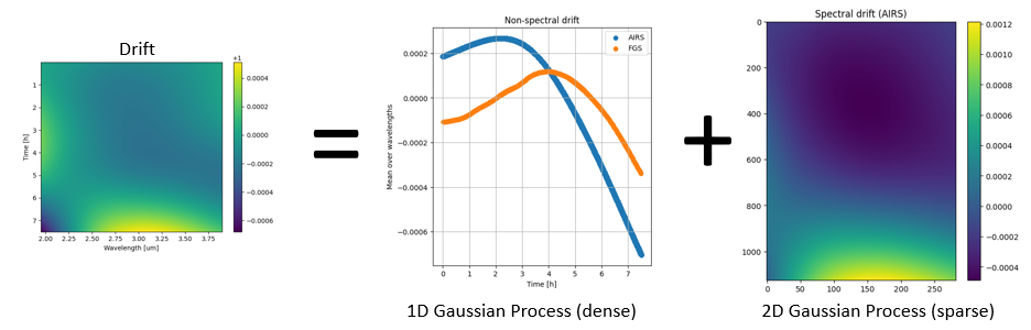\n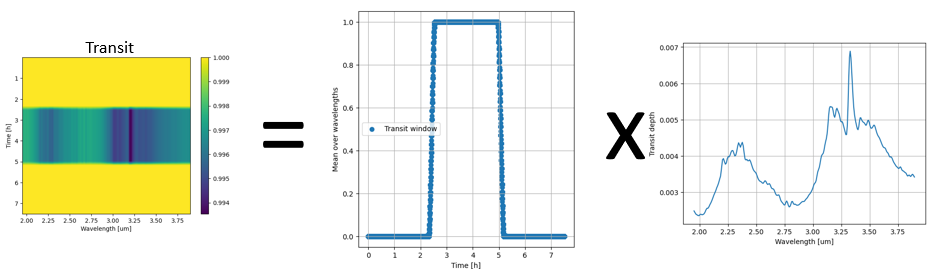\n\n| Prior element | Description | Tuning and hyperparameters | Degrees of freedom |\n| ----------------------------- | ----------------------------------------------------- | ------------------------------------------------------- | -------------------------- |\n| Noise | Uncorrelated Gaussian per time and wavelength | Standard deviations found in preprocessing | 114340 |\n| Star spectrum | Uncorrelated value per wavelength | Not regularized (infinite sigma) | 283 |\n| Drift: 1D | 2x GP over time, 1 for AIRS and 1 for FGS | Tuned on training set | 816 |\n| Drift: 2D | GP over time and wavelength | Tuned on training set | 113928 -> 800 with KISS-GP |\n| Transit window | Fixed function, ingress/egress time and width are fit | Fixed function is found on training set | 3 |\n| Transit depth: mean | Single value | Not regularized | 1 |\n| Transit depth: variation FGS | Single Gaussian value | Standard deviation found on training set | 1 |\n| Transit depth: variation AIRS | GP over wavelength | Tuned on training set | 282 |\n| Transit depth: PCA | Fixed basis functions obtained from PCA analysis | PCA shapes found from an initial rough fit on test data | 1 |\n\nNotes on the details:\n- All GPs use multiple squared-exponential kernels (i.e. they are themselves multiple GPs combined, each with their own fixed length scale). The hyperparameters (sigma values per length scale) are tuned on the training data using various techniques (not currently included in the submission code).\n- We tune one hyperparameter during inference on the test set, per planet: the magnitude of the non-mean part of the transit depth (i.e. the variation and PCA components). This is essentially a scaling applied to all underlying hyperparameters. It is found using maximum likelihood estimation, with a minimum value applied (MLE tends to estimate zero too often).\n- All GPs are solved as dense GPs, except the spectral drift (trying this would lead to a 100k by 100k dense matrix); there we use KISS-GP to sparsify the GP. This works well because the shape is very low-frequent to begin with.\n- There are common shapes between the transit depths per planet, corresponding to specific elements in the atmosphere. I use principal component analysis (PCA) without centering to find these shapes. We can't do this on the training labels, because the test set follows a very different distribution. So the approach is:\n\t- Do a rough fit on all 800 planets using the full model except the PCA shapes.\n\t- Do PCA on the 800 found transit depths (1 or 2 components seems best on the test set; I use 1 for the final submission).\n\t- Redo the fit on all 800 planets, this time including the PCA shapes we just found. This leads to the final reported transit depths.\n- The ingress and egress profiles are a fixed function, found on the training data. We do fit three parameters: the width (i.e. is the ingress abrupt or broad), the ingress time, and the egress time.\n- The star spectrum is an uncorrelated Gaussian per wavelength, constant over time. This is not optimal; I spent a lot of time trying to make use of the fact that different planets for one star have the same star spectrum. This worked quite well on training (+0.005), but was disastrous on test (my final score with it was 0.110).\n- After all the proper Bayesian modeling, some additional fudge factors are applied. These are optimized on the training set, and an additional offset is applied to the test set (found by hill climbing). These are:\n\t- A fixed scaling factor applied to all confidence intervals. For the final submission, this value is around +10%. Its impact on the final score is limited.\n\t- A scaling factor applied to the mean of the transit depth. For the final submission, the mean is multiplied by around 1.0064. This is critical (score would be under 0.7 without), and I have no idea why it's needed... \n\n(EDIT: I since learned from @cnumber that this is due to the fact that I missed a constant background signal; if you turn on include_later_optimization in the code this will be corrected for, and both of these fudge values are disabled)\n\n## Implementation notes\n#### Preprocessing\nMy general preprocessing flow is as follows (details in ariel_support.py):\n- Follow the general preprocessing flow provided by the organizers, with ADC offset sign flipped and several speedups. I also cut off the top 8 and bottom 8 rows of the AIRS signal, which seem to be noisier and anyway contain very little signal.\n- Apply inpainting to remove invalid values (linear interpolation by row). This is quite important, because the jitter causes the signal to move between rows, so the invalids lead to biases.\n- Sum over columns.\n- Estimate ingress and egress time, as well as noise values.\n- Bin over time to reduce data size. I use smaller chunks near the ingress and egress to better capture the profiles there.\n\nI actually have a more involved alternative that includes jitter correction and weighted column summation (to reduce the overall noise). I think these things are needed for optimal performance, but I didn't see enough gain to justify the additional complexity (though I've now seen that I actually some unselected first place submissions with this alternative flow...)\n#### Solving Gaussian Processes\nAs described in the introduction, actually finding the posterior in BI is 'just math' - there's no domain knowledge involved anymore. But we do of course have to implement the math as well. Some notes on this:\n- I made a custom GP toolbox (gp.py). I'm not sure to what degree I could have used the standard ones like GPyTorch, but I wanted to make sure I knew exactly what was going on under the hood.\n- Our prior is nonlinear, i.e. the predicted measurements are not a linear function of the parameters, for example because some prior elements are multiplied rather than added. I deal with this iteratively (7 iterations):\n\t- Pick some suitable starting guess for the parameters.\n\t- Linearize the prior around these parameters.\n\t- Solve the GP with standard methods.\n\t- Use the mean of the posterior as the starting point for the next iteration.\n- The magnitude of the transit depth (the only hyperparameters tuned during inference) is found using gradient descent on the log likelihood (with one update per iteration as described above).\n\n## Conclusion\n\nBy applying Bayesian Inference, we can disentangle the complexity of our model. We can consider each of our physical contributors (noise, drift, transit, etc.) on their own, and separate all that from the actual math of the solver. This leads to a powerful and flexible model - for example, if we need to add additional physics like limb darkening, we only touch one of the elements of the model. Finally, it also provides accurate error estimates - including full covariance matrices per planet, which will be critical for accurate further modeling. I am convinced Bayesian Inference is the way to go for the Ariel project.\n\nIf you have any ideas on how I can increase my impact using these Bayesian methods, or simply recognize the challenge, please get in touch!", "votes": 125 }, { "id": 3034316, "postDate": "2024-11-02T02:23:48.403Z", "content": "Congratulations for your 2nd place!
\nWe also used Gaussian process regresion as part of our solution, but your solution seems to be way more sphisticated compared to our part.
\n\nA scaling factor applied to the mean of the transit depth. For the final submission, the mean is multiplied by around 1.0064. This is critical (score would be under 0.7 without), and I have no idea why it's needed…
\n
This is due to the foreground added during the simulation process in exosim2, which can be removed by estimating the foreground from the [0:8] and [24:32] channels of the sensor.
\nFurther disccusion will be made in our solution post, but to make a long story short, it boosted our score by around 0.010~0.015 compared to when hardcoding the coefficient using values between 1.006 and 1.008.

And foreground subtraction is better than ad hoc calibration factor because it is star dependent; it adds different offset to star-dependent total luminosity.
", "rawMarkdown": "And foreground subtraction is better than ad hoc calibration factor because it is star dependent; it adds different offset to star-dependent total luminosity.", "votes": 1 }, { "id": 3034445, "postDate": "2024-11-02T06:40:02.823Z", "content": "Hm so in terms of my prior, I missed an additive foreground effect (which would be missed by the multiplicative drift term). This might also explain why it was better to remove the outer 8 rows, since they would add more foreground that I don't compensate for. Going to try this out!
\nAny other physics you notice that I missed in my prior?
", "rawMarkdown": "Hm so in terms of my prior, I missed an *additive* foreground effect (which would be missed by the *multiplicative* drift term). This might also explain why it was better to remove the outer 8 rows, since they would add more foreground that I don't compensate for. Going to try this out!\n\nAny other physics you notice that I missed in my prior?" }, { "id": 3034461, "postDate": "2024-11-02T06:56:05.517Z", "content": "Another point you might have missed, is that the gain drift can be expressed by the product of 2 polynomials (probably both 4th order); one in the temporal axis, and one in the wavelength axis, denoted as y_t and y_w in exosim2, resulting in the reduction of parameters.
\n", "rawMarkdown": "Another point you might have missed, is that the gain drift can be expressed by the product of 2 polynomials (probably both 4th order); one in the temporal axis, and one in the wavelength axis, denoted as y_t and y_w in exosim2, resulting in the reduction of parameters.\n\nhttps://github.com/arielmission-space/ExoSim2-public/blob/d94a57c9921538024733b78ff0a2f07e0e5b70a8/exosim/tasks/detector/addGainDrift.py#L135", "votes": 1, "replies": [ { "id": 3034472, "postDate": "2024-11-02T07:11:03.723Z", "content": "I completely missed the exosim clue, that would have helped a lot. But in this case I do think I have an implementation that would be more relevant to the actual mission. Might still try it out.
", "rawMarkdown": "I completely missed the exosim clue, that would have helped a lot. But in this case I do think I have an implementation that would be more relevant to the actual mission. Might still try it out.", "votes": 1 }, { "id": 3034676, "postDate": "2024-11-02T13:02:46.820Z", "content": "I also agree that your solution is more robust than ours.
\nOurs was too \"Kaggleish\" for better or for worse; many hyper-parameters, ensemble of multiple models etc.
\nCongratulations again for your wonderful work!
Thanks, and congratulations on your win!
", "rawMarkdown": "Thanks, and congratulations on your win!", "votes": 2 } ] }, { "id": 3034679, "postDate": "2024-11-02T13:08:53.370Z", "content": "OK since this definitely seems to be true; correcting for this 'foreground focal plane' removes the need to do both mean and sigma biasing. It gains little (~0.001) in CV, but probably much more on LB because there is no fudging needed. Would be nice to see, since it means we're really running the pure Bayesian model. Submitting now…
", "rawMarkdown": "OK since this definitely seems to be true; correcting for this 'foreground focal plane' removes the need to do both mean and sigma biasing. It gains little (~0.001) in CV, but probably much more on LB because there is no fudging needed. Would be nice to see, since it means we're really running the pure Bayesian model. Submitting now...", "votes": 1 }, { "id": 3034718, "postDate": "2024-11-02T14:14:00.727Z", "content": "As you say, we saw a much bigger improvement in LB than in train.
\nVery excited to see how much the scores improve!
I went from 0.740 to 0.745 on private LB with this fix, and to 0.747 if I turn on my advanced jitter correction (briefly mentioned in my solution discussion). That last one's probably just overfitting the private LB though.
", "rawMarkdown": "I went from 0.740 to 0.745 on private LB with this fix, and to 0.747 if I turn on my advanced jitter correction (briefly mentioned in my solution discussion). That last one's probably just overfitting the private LB though.", "votes": 3 }, { "id": 3034996, "postDate": "2024-11-02T22:45:01.390Z", "content": "Nice! This 'fixing' of the predictions by a multiplicative factor bugged me for the entire competition lol
", "rawMarkdown": "Nice! This 'fixing' of the predictions by a multiplicative factor bugged me for the entire competition lol" } ] } ] }, { "id": 3034161, "postDate": "2024-11-01T20:54:01.810Z", "content": "Congratulations on your 2nd place, even if it may look like a lost 1st place now for you.
\nThank you for the write-up. Very clean solution and likely of actual value for the mission!
\nI also saw the drift in wavelength dimension and how 2D gaussian processes are able to catch them, but failed to properly use it. Just applying a fixed drift for all wavelength was always more stable for me. I'll definetely study your code.
\nBy chance, do you have a number how much the extra dimension of freedom boosted your score? And also, how long did the gaussian process fit took per planet. I probably haven't optimized enough, and it was around 20-30 seconds on the kernel hardware.
", "rawMarkdown": "Congratulations on your 2nd place, even if it may look like a lost 1st place now for you. \n\nThank you for the write-up. Very clean solution and likely of actual value for the mission!\n\nI also saw the drift in wavelength dimension and how 2D gaussian processes are able to catch them, but failed to properly use it. Just applying a fixed drift for all wavelength was always more stable for me. I'll definetely study your code. \n\nBy chance, do you have a number how much the extra dimension of freedom boosted your score? And also, how long did the gaussian process fit took per planet. I probably haven't optimized enough, and it was around 20-30 seconds on the kernel hardware.", "votes": 3, "replies": [ { "id": 3034162, "postDate": "2024-11-01T21:00:02.750Z", "content": "\n\nA scaling factor applied to the mean of the transit depth. For the final submission, the mean is multiplied by around 1.0064. This is critical (score would be under 0.7 without), and I have no idea why it's needed…
\n
This is indeed very odd. Certainly not 1-x vs x? Right? And this was on LB and train?
", "rawMarkdown": "> A scaling factor applied to the mean of the transit depth. For the final submission, the mean is multiplied by around 1.0064. This is critical (score would be under 0.7 without), and I have no idea why it's needed…\n\nThis is indeed very odd. Certainly not 1-x vs x? Right? And this was on LB and train?", "votes": 2, "replies": [ { "id": 3034166, "postDate": "2024-11-01T21:05:29.390Z", "content": "What do you mean with 1-x vs x?
\nIndeed, I saw this on both LB and train. I used a slightly different bias on LB, but I'm not sure if the difference is statistically significant. I also saw some improvement by applying a different bias for each star in the LB, but that was almost certainly overfitting.
\nA possible cause is if the ingress/egress profiles are not entirely symmetric (I do assume they are). But I spent quite some time hunting for asymmetries there with no result. Even using symmetric profiles though, I do see the bias I have to apply depending quite a bit on the exact shape I use.
", "rawMarkdown": "What do you mean with 1-x vs x?\n\nIndeed, I saw this on both LB and train. I used a slightly different bias on LB, but I'm not sure if the difference is statistically significant. I also saw some improvement by applying a different bias for each star in the LB, but that was almost certainly overfitting.\n\nA possible cause is if the ingress/egress profiles are not entirely symmetric (I do assume they are). But I spent quite some time hunting for asymmetries there with no result. Even using symmetric profiles though, I do see the bias I have to apply depending quite a bit on the exact shape I use." }, { "id": 3034177, "postDate": "2024-11-01T21:17:56.960Z", "content": "I mean transit depth potentially having two different definitions.
\nE.g. transit at 90 and out of transit is at 100. Now, transit depth can be either defined as 1 - 90/100 or as 100/90 - 1.
", "rawMarkdown": "I mean transit depth potentially having two different definitions. \n\nE.g. transit at 90 and out of transit is at 100. Now, transit depth can be either defined as 1 - 90/100 or as 100/90 - 1." }, { "id": 3034178, "postDate": "2024-11-01T21:20:28.850Z", "content": "Oh good thought. These are easy things to get wrong, but I'm pretty sure my model would report 1-90/100=0.1 in that case. That's also the correct definition, right?
", "rawMarkdown": "Oh good thought. These are easy things to get wrong, but I'm pretty sure my model would report 1-90/100=0.1 in that case. That's also the correct definition, right?" }, { "id": 3034182, "postDate": "2024-11-01T21:23:51.763Z", "content": "I believe the other way is \"correct\", but I was honestly confused a few times, too.
", "rawMarkdown": "I believe the other way is \"correct\", but I was honestly confused a few times, too." }, { "id": 3034190, "postDate": "2024-11-01T21:30:40.743Z", "content": "Hm that would be odd, it would mean a planet blotting out half the light gets a transit depth of 100%. Anyway I'll test this out tomorrow.
", "rawMarkdown": "Hm that would be odd, it would mean a planet blotting out half the light gets a transit depth of 100%. Anyway I'll test this out tomorrow.", "votes": 1 }, { "id": 3034209, "postDate": "2024-11-01T21:52:58.200Z", "content": "I had to do something similar to the transits (added 4e-6). For me, I think it was due to the limb darkening adding a slight bit convexity to the transit section. But it was so small that I could not detect it through the signals.
", "rawMarkdown": "I had to do something similar to the transits (added 4e-6). For me, I think it was due to the limb darkening adding a slight bit convexity to the transit section. But it was so small that I could not detect it through the signals." }, { "id": 3034210, "postDate": "2024-11-01T21:55:34.160Z", "content": "Limb darkening was not modelled in the synthetic data of this competition data.
\nhttps://www.kaggle.com/competitions/ariel-data-challenge-2024/discussion/528683#2964295
\nBut reading that comment again, it seems that deltaF/F (probably F is out of transit here) is actually correct. So, maybe I did that wrong and might explain some bad drops on private LB for older submissions without any model on top. Will also do a review on that tomorrow.
", "rawMarkdown": "Limb darkening was not modelled in the synthetic data of this competition data.\n\nhttps://www.kaggle.com/competitions/ariel-data-challenge-2024/discussion/528683#2964295\n\nBut reading that comment again, it seems that deltaF/F (probably F is out of transit here) is actually correct. So, maybe I did that wrong and might explain some bad drops on private LB for older submissions without any model on top. Will also do a review on that tomorrow." }, { "id": 3034215, "postDate": "2024-11-01T22:01:27.430Z", "content": "I did not know that 😂. Wasted much time trying to deal with limb darkening that didn't exist.
", "rawMarkdown": "I did not know that 😂. Wasted much time trying to deal with limb darkening that didn't exist.", "votes": 1 }, { "id": 3034223, "postDate": "2024-11-01T22:19:58.577Z", "content": "I also tried to find out the reason for such a bias, especially for star 0. I plotted the errors (between true mean planet size and predicted mean planet size) distributions:
\n
One of the hypotheses I was thinking about was \"a big and hot planet and a cold star\". In this case, a planet cannot be considered as totally dark in comparison to its host star, because the ratio \"planet brightness / star brightness\" can be about ~ 1 / 250 (one can use Planck's law for cold stars with temperature 3000 - 4000K and hot planets 500-900K).
\nHowever, it seems like a statistical error, not just for a couple of really hot planets. Probably, the methods we use underestimate the planet size for some reasons?
", "rawMarkdown": "I also tried to find out the reason for such a bias, especially for star 0. I plotted the errors (between true mean planet size and predicted mean planet size) distributions:\n\n\n\nOne of the hypotheses I was thinking about was \"a big and hot planet and a cold star\". In this case, a planet cannot be considered as totally dark in comparison to its host star, because the ratio \"planet brightness / star brightness\" can be about ~ 1 / 250 (one can use [Planck's law](https://en.wikipedia.org/wiki/Planck%27s_law) for cold stars with temperature 3000 - 4000K and hot planets 500-900K).\n\nHowever, it seems like a statistical error, not just for a couple of really hot planets. Probably, the methods we use underestimate the planet size for some reasons?" } ] }, { "id": 3034164, "postDate": "2024-11-01T21:02:29.133Z", "content": "With 'extra dimension' of freedom, you mean the 2D drift? I'm not sure how much that gained; I turned it on before enabling the GP for the transit depth, and as a result the 2D drift 'ate up' all the low-frequent content in the transit depth. So I only started seeing gains when I enabled both, but can't separate the gain. I might still have a look what disabling it does in my latest code, but it's all a bit broken now while I prepare it for release.
\nMy GP fit takes about 30 seconds per planet. That's including both fits (once to establish the PCA, and then the final fit), which both run over mutiple iterations. I think it could be much faster though with the right approximations, but only only went just as far as I needed to with those.
", "rawMarkdown": "With 'extra dimension' of freedom, you mean the 2D drift? I'm not sure how much that gained; I turned it on before enabling the GP for the transit depth, and as a result the 2D drift 'ate up' all the low-frequent content in the transit depth. So I only started seeing gains when I enabled both, but can't separate the gain. I might still have a look what disabling it does in my latest code, but it's all a bit broken now while I prepare it for release.\n\nMy GP fit takes about 30 seconds per planet. That's including both fits (once to establish the PCA, and then the final fit), which both run over mutiple iterations. I think it could be much faster though with the right approximations, but only only went just as far as I needed to with those.", "votes": 2, "replies": [ { "id": 3034170, "postDate": "2024-11-01T21:10:51.337Z", "content": "Yes, the 2D drift. Vs just modeling the drift in the time dimension. Thank you for the time estimate! And did it basically converge at that point or would more iterations even improve local score and potential LB score on better hardware/more time further?
\nCongratulations again
I played around with the number of iterations a bit earlier on and found no gain past 7. But I didn't get around to testing as much as I'd have liked on the final model (I was mainly working on robustness, not expecting a tight finish…)
", "rawMarkdown": "I played around with the number of iterations a bit earlier on and found no gain past 7. But I didn't get around to testing as much as I'd have liked on the final model (I was mainly working on robustness, not expecting a tight finish...)", "votes": 2 } ] } ] }, { "id": 3034147, "postDate": "2024-11-01T20:18:48.187Z", "content": "I cannot understand most of it due to my lacking knowledge, it's very frustrating! 😅😭 Need to learn more bayesian and GP lol
", "rawMarkdown": "I cannot understand most of it due to my lacking knowledge, it's very frustrating! 😅😭 Need to learn more bayesian and GP lol", "votes": 2, "replies": [ { "id": 3034159, "postDate": "2024-11-01T20:45:41.717Z", "content": "You won't regret it if you do learn these! They're very powerful approaches - even in the many cases where true deep learning techniques are needed, they can still boost performance a lot in steps like feature engineering.
", "rawMarkdown": "You won't regret it if you do learn these! They're very powerful approaches - even in the many cases where true deep learning techniques are needed, they can still boost performance a lot in steps like feature engineering. ", "votes": 3, "replies": [ { "id": 3034186, "postDate": "2024-11-01T21:29:09.297Z", "content": "Hi @jeroencottaar. Thank you for the motivation for these approaches. Can you share your code as well ? It would be very very nice for learning purposes.
", "rawMarkdown": "Hi @jeroencottaar. Thank you for the motivation for these approaches. Can you share your code as well ? It would be very very nice for learning purposes." }, { "id": 3034187, "postDate": "2024-11-01T21:30:19.023Z", "content": "Oh i read above it will be available by 3rd November. Thank you so much for this. Also please keep the datasets opened. Like it shouldn't be containing private datasets so that solution can be understood from A to Z.
", "rawMarkdown": "Oh i read above it will be available by 3rd November. Thank you so much for this. Also please keep the datasets opened. Like it shouldn't be containing private datasets so that solution can be understood from A to Z." }, { "id": 3034197, "postDate": "2024-11-01T21:37:23.123Z", "content": "Indeed, I will share everything (think I have to anyway if I want my prize money). So you'll be able to run the code fully including submitting it, and maybe find further improvements!
", "rawMarkdown": "Indeed, I will share everything (think I have to anyway if I want my prize money). So you'll be able to run the code fully including submitting it, and maybe find further improvements!", "votes": 1 }, { "id": 3034205, "postDate": "2024-11-01T21:43:31.653Z", "content": "Thank you so so so much 😀
", "rawMarkdown": "Thank you so so so much 😀" } ] }, { "id": 3034356, "postDate": "2024-11-02T04:01:01.613Z", "rawMarkdown": "", "isDeleted": true, "replies": [ { "id": 3034448, "postDate": "2024-11-02T06:41:45.143Z", "content": "For Bayesian Inference, I only really have a reference if you want to learn it properly: Bayesian Data Analysis 3rd edition by Andrew Gelman and others. Heavy going but you will learn so much. You can find it here, including free PDF download: http://www.stat.columbia.edu/~gelman/book/
\nFor Gaussian Processes I recommend starting at the link I gave above; it's an 8-page paper that covers both the math and the intuition: https://arxiv.org/abs/2009.10862
\nIf you want to go deeper on GPs, go for this book, also available for download: https://gaussianprocess.org/gpml/
", "rawMarkdown": "For Bayesian Inference, I only really have a reference if you want to learn it properly: Bayesian Data Analysis 3rd edition by Andrew Gelman and others. Heavy going but you will learn so much. You can find it here, including free PDF download: http://www.stat.columbia.edu/~gelman/book/\n\nFor Gaussian Processes I recommend starting at the link I gave above; it's an 8-page paper that covers both the math and the intuition: https://arxiv.org/abs/2009.10862\n\nIf you want to go deeper on GPs, go for this book, also available for download: https://gaussianprocess.org/gpml/", "votes": 12 }, { "id": 3034712, "postDate": "2024-11-02T14:07:08.940Z", "rawMarkdown": "", "isDeleted": true }, { "id": 3034719, "postDate": "2024-11-02T14:15:40.277Z", "content": "Feel free to reach out; you should be able to send a message from my Kaggle profile. I can't make any promises on whether I can actually help you though.
", "rawMarkdown": "Feel free to reach out; you should be able to send a message from my Kaggle profile. I can't make any promises on whether I can actually help you though." }, { "id": 3037613, "postDate": "2024-11-05T21:30:21.720Z", "content": "I think you can check out this book, I've had it recommended in a course some time ago, and it has very detailed explanations on a lot of Gaussian concepts as well as Bayesian statistics.
\nhttps://probml.github.io/pml-book/
Thanks, I've indeed had that on my list for a while, but it's rather intimidating…
", "rawMarkdown": "Thanks, I've indeed had that on my list for a while, but it's rather intimidating..." } ] } ] }, { "id": 3272026, "postDate": "2025-08-20T06:17:12.153Z", "content": "This is really cool! It is going to take me a few days just to digest this.
\nAre you using the same approach for Ariel2025 as well? Also, where do I find ariel_gp.py?
", "rawMarkdown": "This is really cool! It is going to take me a few days just to digest this.\n\nAre you using the same approach for Ariel2025 as well? Also, where do I find ariel_gp.py?", "replies": [ { "id": 3274177, "postDate": "2025-08-24T08:55:23.477Z", "content": "For Ariel2025, you'll have to wait and see 😀
\nariel_gp.py (and the other library functions) can be found in the library dataset attached to the notebooks.
", "rawMarkdown": "For Ariel2025, you'll have to wait and see 😀\n\nariel_gp.py (and the other library functions) can be found in the library dataset attached to the notebooks." } ] }, { "id": 3250798, "postDate": "2025-07-19T07:20:21.977Z", "content": "\n\nif we need to add additional physics like limb darkening, we only touch one of the elements of the model.
\n
Hmm…
", "rawMarkdown": "> if we need to add additional physics like limb darkening, we only touch one of the elements of the model.\n\nHmm..." }, { "id": 3043871, "postDate": "2024-11-12T19:05:17.987Z", "content": "Congratulations!
\n\n\nThe hyperparameters (sigma values per length scale) are tuned on the training data using various techniques (not currently included in the submission code).
\n
I would like to learn your solution more and it would help me a lot if you publish the hyperparameter tuning code!
\nIs this similar to that on the test data?
This code would be challenging to share; I put a lot of effort into cleaning up the code, but didn't do that part. It's not in a form that would run on Kaggle.
\nStill, to describe at least what's going on (requires experience with GPs):
\nThank you very much!
\nCan I check if my understanding of the process is right?:tuning the drift hyperparameters then tuning transit depth hyperparameters.
\nI also wonder how the transit window hyperparameters is optimized.
\n\nFit the training planets using the GP, with the transit depth prior replaced by the training labels. For each planet, take a sample from the posterior. Do maximum likelihood estimation for the drift hyperparameters on these samples.
\n
I don’t understand this part.
\nI know simple maximum likelihood estimation, but I don’t know sampling from the posterior and maximum likelihood estimation…
\nI can’t imagine how the likelihood is calculated…
The sampled value is sampled from the distribution that don’t have the hyperparameters we want to optimize, is it right?
", "rawMarkdown": "The sampled value is sampled from the distribution that don’t have the hyperparameters we want to optimize, is it right?" }, { "id": 3044595, "postDate": "2024-11-13T15:19:21.567Z", "content": "It's this basic algorithm for the drift hyperparameters, but unfortunately I don't really have an intuitive explanation, and it might not be easy to match my description above to the general case: https://en.wikipedia.org/wiki/Expectation%E2%80%93maximization_algorithm
\nThe transit hyperparameters are just a single fixed function describing the transit window. Unfortunately the way I find it is a bit complicated, but there isn't really anything of interested going on in there from a machine learning perspective.
", "rawMarkdown": "It's this basic algorithm for the drift hyperparameters, but unfortunately I don't really have an intuitive explanation, and it might not be easy to match my description above to the general case: https://en.wikipedia.org/wiki/Expectation%E2%80%93maximization_algorithm\n\nThe transit hyperparameters are just a single fixed function describing the transit window. Unfortunately the way I find it is a bit complicated, but there isn't really anything of interested going on in there from a machine learning perspective.", "votes": 1 }, { "id": 3044879, "postDate": "2024-11-13T23:31:46.090Z", "content": "Thank you for your kindness to responding to my questions!
\nI’ve learned basics of GP and BI(including EM algorithm), and I’m trying to understand all of your solution(even your code), thinking that this is a wonderful opportunity to learn advanced applications of them!
\nI was thinking of the optimization method for a while, and I noticed that if we use gradient method, we can sample the posterior and do maximum likelihood estimation.
\nBut it seems that your algorithm is similar to EM algorithm though fitting to the general case is difficult.
\nI searched and found the following paper. Is similar method used in this paper?
\nhttps://sipi.usc.edu/~kosko/NEM-FNL-June-2013.pdf
I don't fully follow the paper, but I don't think so. In general I don't think you'd learn much from trying to reproduce my way of fitting hyperparameters; I haven't really put much effort into that part (in general GPs are not too sensitive to the choice of hyperparameters, as long as you're 'close enough'). So you'd probably get more out of trying out different methods you learn about for yourself. You can test the values you find in my submission script; let me know if you manage to find improvements on the score!
", "rawMarkdown": "I don't fully follow the paper, but I don't think so. In general I don't think you'd learn much from trying to reproduce my way of fitting hyperparameters; I haven't really put much effort into that part (in general GPs are not too sensitive to the choice of hyperparameters, as long as you're 'close enough'). So you'd probably get more out of trying out different methods you learn about for yourself. You can test the values you find in my submission script; let me know if you manage to find improvements on the score!", "votes": 1 } ] } ] }, { "id": 3039523, "postDate": "2024-11-08T06:20:31.893Z", "content": "Thanks for sharing you experience it means a lot for the beginners like me? Looking forward to learn from you.
", "rawMarkdown": "Thanks for sharing you experience it means a lot for the beginners like me? Looking forward to learn from you." }, { "id": 3036415, "postDate": "2024-11-04T14:36:35.623Z", "content": "Thanks for sharing this insightful post. @jeroencottaar I invite you to try out this competition as well
", "rawMarkdown": "Thanks for sharing this insightful post. @jeroencottaar I invite you to try out [this](https://www.kaggle.com/competitions/airs-ai-in-respiratory-sounds) competition as well", "replies": [ { "id": 3036429, "postDate": "2024-11-04T14:42:45.820Z", "content": "Thanks, looks cool but I really have to cut down on my Kaggling for a while 😀
", "rawMarkdown": "Thanks, looks cool but I really have to cut down on my Kaggling for a while 😀", "replies": [ { "id": 3036439, "postDate": "2024-11-04T14:50:27.680Z", "content": "Oh Okay. Would have loved to have your thoughts and insights boost fellow competitors strategies.
", "rawMarkdown": "Oh Okay. Would have loved to have your thoughts and insights boost fellow competitors strategies." } ] } ] }, { "id": 3035766, "postDate": "2024-11-03T20:36:56.753Z", "content": "Thanks. Great Bayesian Approach. They often do well in these types of competitions, but indeed not often seen in deep learning times:
\nOne the previous competitions: https://homepages.inf.ed.ac.uk/imurray2/pub/12kaggle_dark/
\nhttps://web.archive.org/web/20131210101140/timsalimans.com/observing-dark-worlds/
These approaches do well outside competitions too, but I'm having trouble getting them accepted in my professional life…
\nThanks for pointing out these earlier Bayesian solutions. I'll try to get in touch with these people to see if they have any insights where I can go from here (in fact, let's see if I get their attention here: @timsalimans @iain2476).
", "rawMarkdown": "These approaches do well outside competitions too, but I'm having trouble getting them accepted in my professional life...\n\nThanks for pointing out these earlier Bayesian solutions. I'll try to get in touch with these people to see if they have any insights where I can go from here (in fact, let's see if I get their attention here: @timsalimans @iain2476)." } ] }, { "id": 3035195, "postDate": "2024-11-03T05:56:26.597Z", "content": "Well done on your achievement, and I appreciate you sharing this insightful write-up!
", "rawMarkdown": "Well done on your achievement, and I appreciate you sharing this insightful write-up!" }, { "id": 3034814, "postDate": "2024-11-02T16:50:15.850Z", "content": "Congratulations!
\nCould you please dive a little deeper into the domain-specific terminology? Namely, I'm confused about what is \"drift\" and \"ingress and egress time\"
I use the term drift to simply indicate any slow changes over time or wavelength in the detector signal.
\nThe ingress time is when the planet starts its transit (i.e. is at the edge of the star), and the egress time when it ends it.
", "rawMarkdown": "I use the term drift to simply indicate any slow changes over time or wavelength in the detector signal.\n\nThe ingress time is when the planet starts its transit (i.e. is at the edge of the star), and the egress time when it ends it.", "votes": 1 } ] }, { "id": 3034694, "postDate": "2024-11-02T13:39:12.530Z", "content": "Congratulations! I was under the impression that Data Science and AI had only to do with Deep-learning and tree based models, very inspiring and exciting that other methods out there produce so competitive results, i will definatelly try to study them!
\nPS: We need to make some Data Science meet-up in Eindhoven!
", "rawMarkdown": "Congratulations! I was under the impression that Data Science and AI had only to do with Deep-learning and tree based models, very inspiring and exciting that other methods out there produce so competitive results, i will definatelly try to study them!\n\nPS: We need to make some Data Science meet-up in Eindhoven!" }, { "id": 3034428, "postDate": "2024-11-02T06:08:52.260Z", "content": "Congratulations for your win and and thanks for sharing interesting write up.
\nJust curious to know if general aspects of physics/signal processing is adequate or you needed any other specific information on space domain for building the priors?
\n'including full covariance matrices per planet' -
\nWhat was the runtime of your submission?
Looking forward to your code. Thanks and Congrats again.
", "rawMarkdown": "Congratulations for your win and and thanks for sharing interesting write up.\n\nJust curious to know if general aspects of physics/signal processing is adequate or you needed any other specific information on space domain for building the priors? \n\n'including full covariance matrices per planet' - \nWhat was the runtime of your submission?\n\nLooking forward to your code. Thanks and Congrats again.", "replies": [ { "id": 3034451, "postDate": "2024-11-02T06:43:45.893Z", "content": "I didn't spend too much time reading literature (which was probably a mistake); I found most of the prior from the data itself. The way this works is that you do Bayesian Inference, and then check that your posterior is consistent with your prior. For example, if you miss drift you will see that your noise in the posterior ends up correlated. This is a clue that you're missing something in the prior. By iterating in this way you can improve the prior, and that's how I ended up with the final prior.
\nMy submission takes about 8 hours.
", "rawMarkdown": "I didn't spend too much time reading literature (which was probably a mistake); I found most of the prior from the data itself. The way this works is that you do Bayesian Inference, and then check that your posterior is consistent with your prior. For example, if you miss drift you will see that your noise in the posterior ends up correlated. This is a clue that you're missing something in the prior. By iterating in this way you can improve the prior, and that's how I ended up with the final prior.\n\nMy submission takes about 8 hours.", "votes": 1 } ] }, { "id": 3034263, "postDate": "2024-11-02T00:03:17.940Z", "content": "Thanks for sharing, Much useful. Waiting for the code also.👍
\nand Congratulations on win 🏅🎉
Oh, wow! I've seen similar techniques in articles and tried to apply them to this problem. However, I probably didn't put in enough effort, couldn't find the right parameters, and of course, I don't have the same level of expertise as you do. Great work and excellent description! Congratulations on your victory!
", "rawMarkdown": "Oh, wow! I've seen similar techniques in articles and tried to apply them to this problem. However, I probably didn't put in enough effort, couldn't find the right parameters, and of course, I don't have the same level of expertise as you do. Great work and excellent description! Congratulations on your victory!\n" }, { "id": 3034200, "postDate": "2024-11-01T21:41:23.853Z", "rawMarkdown": "", "isDeleted": true } ], "comments": [ { "id": 3034316, "author_name": "c-number", "author_url": "", "post_date": "2024-11-02T02:23:48.403000", "content": "Congratulations for your 2nd place!
\nWe also used Gaussian process regresion as part of our solution, but your solution seems to be way more sphisticated compared to our part.
\n\nA scaling factor applied to the mean of the transit depth. For the final submission, the mean is multiplied by around 1.0064. This is critical (score would be under 0.7 without), and I have no idea why it's needed…
\n
This is due to the foreground added during the simulation process in exosim2, which can be removed by estimating the foreground from the [0:8] and [24:32] channels of the sensor.
\nFurther disccusion will be made in our solution post, but to make a long story short, it boosted our score by around 0.010~0.015 compared to when hardcoding the coefficient using values between 1.006 and 1.008.
And foreground subtraction is better than ad hoc calibration factor because it is star dependent; it adds different offset to star-dependent total luminosity.
", "votes": 1, "replies": [] }, { "id": 3034445, "author_name": "Jeroen Cottaar", "author_url": "", "post_date": "2024-11-02T06:40:02.823000", "content": "Hm so in terms of my prior, I missed an additive foreground effect (which would be missed by the multiplicative drift term). This might also explain why it was better to remove the outer 8 rows, since they would add more foreground that I don't compensate for. Going to try this out!
\nAny other physics you notice that I missed in my prior?
", "votes": 0, "replies": [] }, { "id": 3034461, "author_name": "c-number", "author_url": "", "post_date": "2024-11-02T06:56:05.517000", "content": "Another point you might have missed, is that the gain drift can be expressed by the product of 2 polynomials (probably both 4th order); one in the temporal axis, and one in the wavelength axis, denoted as y_t and y_w in exosim2, resulting in the reduction of parameters.
\n", "votes": 1, "replies": [ { "id": 3034472, "author_name": "Jeroen Cottaar", "author_url": "", "post_date": "2024-11-02T07:11:03.723000", "content": "I completely missed the exosim clue, that would have helped a lot. But in this case I do think I have an implementation that would be more relevant to the actual mission. Might still try it out.
", "votes": 1, "replies": [] }, { "id": 3034676, "author_name": "c-number", "author_url": "", "post_date": "2024-11-02T13:02:46.820000", "content": "I also agree that your solution is more robust than ours.
\nOurs was too \"Kaggleish\" for better or for worse; many hyper-parameters, ensemble of multiple models etc.
\nCongratulations again for your wonderful work!
Thanks, and congratulations on your win!
", "votes": 2, "replies": [] } ] }, { "id": 3034679, "author_name": "Jeroen Cottaar", "author_url": "", "post_date": "2024-11-02T13:08:53.370000", "content": "OK since this definitely seems to be true; correcting for this 'foreground focal plane' removes the need to do both mean and sigma biasing. It gains little (~0.001) in CV, but probably much more on LB because there is no fudging needed. Would be nice to see, since it means we're really running the pure Bayesian model. Submitting now…
", "votes": 1, "replies": [] }, { "id": 3034718, "author_name": "c-number", "author_url": "", "post_date": "2024-11-02T14:14:00.727000", "content": "As you say, we saw a much bigger improvement in LB than in train.
\nVery excited to see how much the scores improve!
I went from 0.740 to 0.745 on private LB with this fix, and to 0.747 if I turn on my advanced jitter correction (briefly mentioned in my solution discussion). That last one's probably just overfitting the private LB though.
", "votes": 3, "replies": [] }, { "id": 3034996, "author_name": "greySnow", "author_url": "", "post_date": "2024-11-02T22:45:01.390000", "content": "Nice! This 'fixing' of the predictions by a multiplicative factor bugged me for the entire competition lol
", "votes": 0, "replies": [] } ] } ] }, { "id": 3034161, "author_name": "Pascal Pfeiffer", "author_url": "", "post_date": "2024-11-01T20:54:01.810000", "content": "Congratulations on your 2nd place, even if it may look like a lost 1st place now for you.
\nThank you for the write-up. Very clean solution and likely of actual value for the mission!
\nI also saw the drift in wavelength dimension and how 2D gaussian processes are able to catch them, but failed to properly use it. Just applying a fixed drift for all wavelength was always more stable for me. I'll definetely study your code.
\nBy chance, do you have a number how much the extra dimension of freedom boosted your score? And also, how long did the gaussian process fit took per planet. I probably haven't optimized enough, and it was around 20-30 seconds on the kernel hardware.
", "votes": 3, "replies": [ { "id": 3034162, "author_name": "Pascal Pfeiffer", "author_url": "", "post_date": "2024-11-01T21:00:02.750000", "content": "\n\nA scaling factor applied to the mean of the transit depth. For the final submission, the mean is multiplied by around 1.0064. This is critical (score would be under 0.7 without), and I have no idea why it's needed…
\n
This is indeed very odd. Certainly not 1-x vs x? Right? And this was on LB and train?
", "votes": 2, "replies": [ { "id": 3034166, "author_name": "Jeroen Cottaar", "author_url": "", "post_date": "2024-11-01T21:05:29.390000", "content": "What do you mean with 1-x vs x?
\nIndeed, I saw this on both LB and train. I used a slightly different bias on LB, but I'm not sure if the difference is statistically significant. I also saw some improvement by applying a different bias for each star in the LB, but that was almost certainly overfitting.
\nA possible cause is if the ingress/egress profiles are not entirely symmetric (I do assume they are). But I spent quite some time hunting for asymmetries there with no result. Even using symmetric profiles though, I do see the bias I have to apply depending quite a bit on the exact shape I use.
", "votes": 0, "replies": [] }, { "id": 3034177, "author_name": "Pascal Pfeiffer", "author_url": "", "post_date": "2024-11-01T21:17:56.960000", "content": "I mean transit depth potentially having two different definitions.
\nE.g. transit at 90 and out of transit is at 100. Now, transit depth can be either defined as 1 - 90/100 or as 100/90 - 1.
", "votes": 0, "replies": [] }, { "id": 3034178, "author_name": "Jeroen Cottaar", "author_url": "", "post_date": "2024-11-01T21:20:28.850000", "content": "Oh good thought. These are easy things to get wrong, but I'm pretty sure my model would report 1-90/100=0.1 in that case. That's also the correct definition, right?
", "votes": 0, "replies": [] }, { "id": 3034182, "author_name": "Pascal Pfeiffer", "author_url": "", "post_date": "2024-11-01T21:23:51.763000", "content": "I believe the other way is \"correct\", but I was honestly confused a few times, too.
", "votes": 0, "replies": [] }, { "id": 3034190, "author_name": "Jeroen Cottaar", "author_url": "", "post_date": "2024-11-01T21:30:40.743000", "content": "Hm that would be odd, it would mean a planet blotting out half the light gets a transit depth of 100%. Anyway I'll test this out tomorrow.
", "votes": 1, "replies": [] }, { "id": 3034209, "author_name": "JungleBeastDS", "author_url": "", "post_date": "2024-11-01T21:52:58.200000", "content": "I had to do something similar to the transits (added 4e-6). For me, I think it was due to the limb darkening adding a slight bit convexity to the transit section. But it was so small that I could not detect it through the signals.
", "votes": 0, "replies": [] }, { "id": 3034210, "author_name": "Pascal Pfeiffer", "author_url": "", "post_date": "2024-11-01T21:55:34.160000", "content": "Limb darkening was not modelled in the synthetic data of this competition data.
\nhttps://www.kaggle.com/competitions/ariel-data-challenge-2024/discussion/528683#2964295
\nBut reading that comment again, it seems that deltaF/F (probably F is out of transit here) is actually correct. So, maybe I did that wrong and might explain some bad drops on private LB for older submissions without any model on top. Will also do a review on that tomorrow.
", "votes": 0, "replies": [] }, { "id": 3034215, "author_name": "JungleBeastDS", "author_url": "", "post_date": "2024-11-01T22:01:27.430000", "content": "I did not know that 😂. Wasted much time trying to deal with limb darkening that didn't exist.
", "votes": 1, "replies": [] }, { "id": 3034223, "author_name": "gromml", "author_url": "", "post_date": "2024-11-01T22:19:58.577000", "content": "I also tried to find out the reason for such a bias, especially for star 0. I plotted the errors (between true mean planet size and predicted mean planet size) distributions:
\n
One of the hypotheses I was thinking about was \"a big and hot planet and a cold star\". In this case, a planet cannot be considered as totally dark in comparison to its host star, because the ratio \"planet brightness / star brightness\" can be about ~ 1 / 250 (one can use Planck's law for cold stars with temperature 3000 - 4000K and hot planets 500-900K).
\nHowever, it seems like a statistical error, not just for a couple of really hot planets. Probably, the methods we use underestimate the planet size for some reasons?
", "votes": 0, "replies": [] } ] }, { "id": 3034164, "author_name": "Jeroen Cottaar", "author_url": "", "post_date": "2024-11-01T21:02:29.133000", "content": "With 'extra dimension' of freedom, you mean the 2D drift? I'm not sure how much that gained; I turned it on before enabling the GP for the transit depth, and as a result the 2D drift 'ate up' all the low-frequent content in the transit depth. So I only started seeing gains when I enabled both, but can't separate the gain. I might still have a look what disabling it does in my latest code, but it's all a bit broken now while I prepare it for release.
\nMy GP fit takes about 30 seconds per planet. That's including both fits (once to establish the PCA, and then the final fit), which both run over mutiple iterations. I think it could be much faster though with the right approximations, but only only went just as far as I needed to with those.
", "votes": 2, "replies": [ { "id": 3034170, "author_name": "Pascal Pfeiffer", "author_url": "", "post_date": "2024-11-01T21:10:51.337000", "content": "Yes, the 2D drift. Vs just modeling the drift in the time dimension. Thank you for the time estimate! And did it basically converge at that point or would more iterations even improve local score and potential LB score on better hardware/more time further?
\nCongratulations again
I played around with the number of iterations a bit earlier on and found no gain past 7. But I didn't get around to testing as much as I'd have liked on the final model (I was mainly working on robustness, not expecting a tight finish…)
", "votes": 2, "replies": [] } ] } ] }, { "id": 3034147, "author_name": "greySnow", "author_url": "", "post_date": "2024-11-01T20:18:48.187000", "content": "I cannot understand most of it due to my lacking knowledge, it's very frustrating! 😅😭 Need to learn more bayesian and GP lol
", "votes": 2, "replies": [ { "id": 3034159, "author_name": "Jeroen Cottaar", "author_url": "", "post_date": "2024-11-01T20:45:41.717000", "content": "You won't regret it if you do learn these! They're very powerful approaches - even in the many cases where true deep learning techniques are needed, they can still boost performance a lot in steps like feature engineering.
", "votes": 3, "replies": [ { "id": 3034186, "author_name": "JamshaidSohail", "author_url": "", "post_date": "2024-11-01T21:29:09.297000", "content": "Hi @jeroencottaar. Thank you for the motivation for these approaches. Can you share your code as well ? It would be very very nice for learning purposes.
", "votes": 0, "replies": [] }, { "id": 3034187, "author_name": "JamshaidSohail", "author_url": "", "post_date": "2024-11-01T21:30:19.023000", "content": "Oh i read above it will be available by 3rd November. Thank you so much for this. Also please keep the datasets opened. Like it shouldn't be containing private datasets so that solution can be understood from A to Z.
", "votes": 0, "replies": [] }, { "id": 3034197, "author_name": "Jeroen Cottaar", "author_url": "", "post_date": "2024-11-01T21:37:23.123000", "content": "Indeed, I will share everything (think I have to anyway if I want my prize money). So you'll be able to run the code fully including submitting it, and maybe find further improvements!
", "votes": 1, "replies": [] }, { "id": 3034205, "author_name": "JamshaidSohail", "author_url": "", "post_date": "2024-11-01T21:43:31.653000", "content": "Thank you so so so much 😀
", "votes": 0, "replies": [] } ] }, { "id": 3034356, "author_name": "", "author_url": "", "post_date": "2024-11-02T04:01:01.613000", "content": "", "votes": 0, "replies": [ { "id": 3034448, "author_name": "Jeroen Cottaar", "author_url": "", "post_date": "2024-11-02T06:41:45.143000", "content": "For Bayesian Inference, I only really have a reference if you want to learn it properly: Bayesian Data Analysis 3rd edition by Andrew Gelman and others. Heavy going but you will learn so much. You can find it here, including free PDF download: http://www.stat.columbia.edu/~gelman/book/
\nFor Gaussian Processes I recommend starting at the link I gave above; it's an 8-page paper that covers both the math and the intuition: https://arxiv.org/abs/2009.10862
\nIf you want to go deeper on GPs, go for this book, also available for download: https://gaussianprocess.org/gpml/
", "votes": 12, "replies": [] }, { "id": 3034712, "author_name": "", "author_url": "", "post_date": "2024-11-02T14:07:08.940000", "content": "", "votes": 0, "replies": [] }, { "id": 3034719, "author_name": "Jeroen Cottaar", "author_url": "", "post_date": "2024-11-02T14:15:40.277000", "content": "Feel free to reach out; you should be able to send a message from my Kaggle profile. I can't make any promises on whether I can actually help you though.
", "votes": 0, "replies": [] }, { "id": 3037613, "author_name": "Etienne Bardet", "author_url": "", "post_date": "2024-11-05T21:30:21.720000", "content": "I think you can check out this book, I've had it recommended in a course some time ago, and it has very detailed explanations on a lot of Gaussian concepts as well as Bayesian statistics.
\nhttps://probml.github.io/pml-book/
Thanks, I've indeed had that on my list for a while, but it's rather intimidating…
", "votes": 0, "replies": [] } ] } ] }, { "id": 3272026, "author_name": "Saugat Kandel", "author_url": "", "post_date": "2025-08-20T06:17:12.153000", "content": "This is really cool! It is going to take me a few days just to digest this.
\nAre you using the same approach for Ariel2025 as well? Also, where do I find ariel_gp.py?
", "votes": 0, "replies": [ { "id": 3274177, "author_name": "Jeroen Cottaar", "author_url": "", "post_date": "2025-08-24T08:55:23.477000", "content": "For Ariel2025, you'll have to wait and see 😀
\nariel_gp.py (and the other library functions) can be found in the library dataset attached to the notebooks.
", "votes": 0, "replies": [] } ] }, { "id": 3250798, "author_name": "c-number", "author_url": "", "post_date": "2025-07-19T07:20:21.977000", "content": "\n\nif we need to add additional physics like limb darkening, we only touch one of the elements of the model.
\n
Hmm…
", "votes": 0, "replies": [] }, { "id": 3043871, "author_name": "moto", "author_url": "", "post_date": "2024-11-12T19:05:17.987000", "content": "Congratulations!
\n\n\nThe hyperparameters (sigma values per length scale) are tuned on the training data using various techniques (not currently included in the submission code).
\n
I would like to learn your solution more and it would help me a lot if you publish the hyperparameter tuning code!
\nIs this similar to that on the test data?
This code would be challenging to share; I put a lot of effort into cleaning up the code, but didn't do that part. It's not in a form that would run on Kaggle.
\nStill, to describe at least what's going on (requires experience with GPs):
\nThank you very much!
\nCan I check if my understanding of the process is right?:tuning the drift hyperparameters then tuning transit depth hyperparameters.
\nI also wonder how the transit window hyperparameters is optimized.
\n\nFit the training planets using the GP, with the transit depth prior replaced by the training labels. For each planet, take a sample from the posterior. Do maximum likelihood estimation for the drift hyperparameters on these samples.
\n
I don’t understand this part.
\nI know simple maximum likelihood estimation, but I don’t know sampling from the posterior and maximum likelihood estimation…
\nI can’t imagine how the likelihood is calculated…
The sampled value is sampled from the distribution that don’t have the hyperparameters we want to optimize, is it right?
", "votes": 0, "replies": [] }, { "id": 3044595, "author_name": "Jeroen Cottaar", "author_url": "", "post_date": "2024-11-13T15:19:21.567000", "content": "It's this basic algorithm for the drift hyperparameters, but unfortunately I don't really have an intuitive explanation, and it might not be easy to match my description above to the general case: https://en.wikipedia.org/wiki/Expectation%E2%80%93maximization_algorithm
\nThe transit hyperparameters are just a single fixed function describing the transit window. Unfortunately the way I find it is a bit complicated, but there isn't really anything of interested going on in there from a machine learning perspective.
", "votes": 1, "replies": [] }, { "id": 3044879, "author_name": "moto", "author_url": "", "post_date": "2024-11-13T23:31:46.090000", "content": "Thank you for your kindness to responding to my questions!
\nI’ve learned basics of GP and BI(including EM algorithm), and I’m trying to understand all of your solution(even your code), thinking that this is a wonderful opportunity to learn advanced applications of them!
\nI was thinking of the optimization method for a while, and I noticed that if we use gradient method, we can sample the posterior and do maximum likelihood estimation.
\nBut it seems that your algorithm is similar to EM algorithm though fitting to the general case is difficult.
\nI searched and found the following paper. Is similar method used in this paper?
\nhttps://sipi.usc.edu/~kosko/NEM-FNL-June-2013.pdf
I don't fully follow the paper, but I don't think so. In general I don't think you'd learn much from trying to reproduce my way of fitting hyperparameters; I haven't really put much effort into that part (in general GPs are not too sensitive to the choice of hyperparameters, as long as you're 'close enough'). So you'd probably get more out of trying out different methods you learn about for yourself. You can test the values you find in my submission script; let me know if you manage to find improvements on the score!
", "votes": 1, "replies": [] } ] } ] }, { "id": 3039523, "author_name": "Tanishk Patil", "author_url": "", "post_date": "2024-11-08T06:20:31.893000", "content": "Thanks for sharing you experience it means a lot for the beginners like me? Looking forward to learn from you.
", "votes": 0, "replies": [] }, { "id": 3036415, "author_name": "Himanshu Kaushik", "author_url": "", "post_date": "2024-11-04T14:36:35.623000", "content": "Thanks for sharing this insightful post. @jeroencottaar I invite you to try out this competition as well
", "votes": 0, "replies": [ { "id": 3036429, "author_name": "Jeroen Cottaar", "author_url": "", "post_date": "2024-11-04T14:42:45.820000", "content": "Thanks, looks cool but I really have to cut down on my Kaggling for a while 😀
", "votes": 0, "replies": [ { "id": 3036439, "author_name": "Himanshu Kaushik", "author_url": "", "post_date": "2024-11-04T14:50:27.680000", "content": "Oh Okay. Would have loved to have your thoughts and insights boost fellow competitors strategies.
", "votes": 0, "replies": [] } ] } ] }, { "id": 3035766, "author_name": "Maxim Shatskiy", "author_url": "", "post_date": "2024-11-03T20:36:56.753000", "content": "Thanks. Great Bayesian Approach. They often do well in these types of competitions, but indeed not often seen in deep learning times:
\nOne the previous competitions: https://homepages.inf.ed.ac.uk/imurray2/pub/12kaggle_dark/
\nhttps://web.archive.org/web/20131210101140/timsalimans.com/observing-dark-worlds/
These approaches do well outside competitions too, but I'm having trouble getting them accepted in my professional life…
\nThanks for pointing out these earlier Bayesian solutions. I'll try to get in touch with these people to see if they have any insights where I can go from here (in fact, let's see if I get their attention here: @timsalimans @iain2476).
", "votes": 0, "replies": [] } ] }, { "id": 3035195, "author_name": "Humayra Khanom Rime", "author_url": "", "post_date": "2024-11-03T05:56:26.597000", "content": "Well done on your achievement, and I appreciate you sharing this insightful write-up!
", "votes": 0, "replies": [] }, { "id": 3034814, "author_name": "Andrey", "author_url": "", "post_date": "2024-11-02T16:50:15.850000", "content": "Congratulations!
\nCould you please dive a little deeper into the domain-specific terminology? Namely, I'm confused about what is \"drift\" and \"ingress and egress time\"
I use the term drift to simply indicate any slow changes over time or wavelength in the detector signal.
\nThe ingress time is when the planet starts its transit (i.e. is at the edge of the star), and the egress time when it ends it.
", "votes": 1, "replies": [] } ] }, { "id": 3034694, "author_name": "Vasilis", "author_url": "", "post_date": "2024-11-02T13:39:12.530000", "content": "Congratulations! I was under the impression that Data Science and AI had only to do with Deep-learning and tree based models, very inspiring and exciting that other methods out there produce so competitive results, i will definatelly try to study them!
\nPS: We need to make some Data Science meet-up in Eindhoven!
", "votes": 0, "replies": [] }, { "id": 3034428, "author_name": "Viji", "author_url": "", "post_date": "2024-11-02T06:08:52.260000", "content": "Congratulations for your win and and thanks for sharing interesting write up.
\nJust curious to know if general aspects of physics/signal processing is adequate or you needed any other specific information on space domain for building the priors?
\n'including full covariance matrices per planet' -
\nWhat was the runtime of your submission?
Looking forward to your code. Thanks and Congrats again.
", "votes": 0, "replies": [ { "id": 3034451, "author_name": "Jeroen Cottaar", "author_url": "", "post_date": "2024-11-02T06:43:45.893000", "content": "I didn't spend too much time reading literature (which was probably a mistake); I found most of the prior from the data itself. The way this works is that you do Bayesian Inference, and then check that your posterior is consistent with your prior. For example, if you miss drift you will see that your noise in the posterior ends up correlated. This is a clue that you're missing something in the prior. By iterating in this way you can improve the prior, and that's how I ended up with the final prior.
\nMy submission takes about 8 hours.
", "votes": 1, "replies": [] } ] }, { "id": 3034263, "author_name": "Vidyavrat Taak", "author_url": "", "post_date": "2024-11-02T00:03:17.940000", "content": "Thanks for sharing, Much useful. Waiting for the code also.👍
\nand Congratulations on win 🏅🎉
Oh, wow! I've seen similar techniques in articles and tried to apply them to this problem. However, I probably didn't put in enough effort, couldn't find the right parameters, and of course, I don't have the same level of expertise as you do. Great work and excellent description! Congratulations on your victory!
", "votes": 0, "replies": [] }, { "id": 3034200, "author_name": "", "author_url": "", "post_date": "2024-11-01T21:41:23.853000", "content": "", "votes": 0, "replies": [] } ], "raw_markdown_by_id": { "3034133": "**Link to submission code**: https://www.kaggle.com/code/jeroencottaar/ariel-2nd-place-submission-notebook \n**Link to visualization code**: https://www.kaggle.com/code/jeroencottaar/ariel-2nd-place-visualization-notebook\n\n**Looking for opportunities and guidance**: the Bayesian Inference approach I describe below is good for much more than competitions - it's applicable to many real-world problems, and is underused in our deep-learning-oriented times. I believe I can meaningfully impact our world with my knowledge of these techniques, but am currently struggling to find the right path in my career to achieve this. If you have insights on how to make a more significant impact with Bayesian methods, I’d be grateful for any guidance, perhaps in a mentorship capacity.\n\n## Introduction\n\nTransit analysis is the most common method for detecting and studying exoplanets. A transit occurs when a planet crosses in front of its star relative to Earth, obscuring part of the starlight. By observing how much the light is reduced (the transit depth) as a function of wavelength, we can learn the properties of the planet. But with a tiny planet passing in front of a huge star, this problem has a very low signal to noise ratio. The challenge to us: find the transit depth, including confidence intervals, from synthetic raw spectroscopic signals as the Ariel satellite might see them in the future (For a more extensive overview, see https://www.kaggle.com/competitions/ariel-data-challenge-2024/overview).\n\n\n\nMy solution to this challenge is built on the related concepts of **Bayesian Inference** and **Gaussian Processes**.\n\n**Bayesian Inference** (BI) is a powerful statistical approach, based around defining a *prior* (a statistical belief about reality) and *observations* (some form of new information). Using Bayes' law, we then combined these to find the *posterior* (an updated belief about reality). In our case, this means:\n- **Prior**: a description of the physics that affect the final measured signal, describing for example detector noise, drift, and the transit behavior (including the transit depth itself) as formal distributions.\n- **Observations**: the provided measurements.\n- **Posterior**: a breakdown of the observations into the various elements defined in the prior (see figure below). From this we can simply read out the desired transit depth. Importantly, the posterior is not just a single point, it's a distribution. By taking samples from this distribution we can find the required confidence intervals (and even full covariance matrices, although that is not asked of us here).\n\nTo me, the most attractive element of BI is how it lets us split our physical thinking from our solver. All our domain knowledge goes into defining the prior, where we can consider one physical element at a time; doing the actual Bayesian Inference to find the posterior is then 'just math'. Not necessarily easy math - but it's entirely separate from our domain knowledge. \n\nThe figure below shows how one example transit is split in the posterior:\n\n\n\nSeveral of our prior elements are smooth functions; for example, transit depth is a function of wavelength, drift is a function of wavelength and time, etc. This means that we need to describe a distribution of functions in the prior. **Gaussian Processes** (GPs) are a natural way to do this. GPs are non-parametric methods, meaning they do not rely on a fixed set of basis functions. Instead, they allow any function, but assign different probabilities to different functions. For example, a low-frequent drift is more likely than a high-frequent one. An excellent starting point to learn GPs is https://arxiv.org/abs/2009.10862\n\nIn my post here, I'll mainly focus on providing the details of the model, which in the BI framework just means describing the prior. At the end I'll cover some odds and ends (preprocessing and how we actually do the BI math).\n## Prior definition\n\nIn this section I'll provide some visual breakdowns, an overview of the various elements, and some notes. You will see references to separate sensors (AIRS and FGS), but I don't really discuss my use of these sensors; The AIRS is the main sensor (the spectroscope). This section assumes familiarity with GPs, but hopefully you can get the gist of it in any case. If you want to know all the details, you'll have to go into the code (ariel_gp.py). \n\n\n\n\n| Prior element | Description | Tuning and hyperparameters | Degrees of freedom |\n| ----------------------------- | ----------------------------------------------------- | ------------------------------------------------------- | -------------------------- |\n| Noise | Uncorrelated Gaussian per time and wavelength | Standard deviations found in preprocessing | 114340 |\n| Star spectrum | Uncorrelated value per wavelength | Not regularized (infinite sigma) | 283 |\n| Drift: 1D | 2x GP over time, 1 for AIRS and 1 for FGS | Tuned on training set | 816 |\n| Drift: 2D | GP over time and wavelength | Tuned on training set | 113928 -> 800 with KISS-GP |\n| Transit window | Fixed function, ingress/egress time and width are fit | Fixed function is found on training set | 3 |\n| Transit depth: mean | Single value | Not regularized | 1 |\n| Transit depth: variation FGS | Single Gaussian value | Standard deviation found on training set | 1 |\n| Transit depth: variation AIRS | GP over wavelength | Tuned on training set | 282 |\n| Transit depth: PCA | Fixed basis functions obtained from PCA analysis | PCA shapes found from an initial rough fit on test data | 1 |\n\nNotes on the details:\n- All GPs use multiple squared-exponential kernels (i.e. they are themselves multiple GPs combined, each with their own fixed length scale). The hyperparameters (sigma values per length scale) are tuned on the training data using various techniques (not currently included in the submission code).\n- We tune one hyperparameter during inference on the test set, per planet: the magnitude of the non-mean part of the transit depth (i.e. the variation and PCA components). This is essentially a scaling applied to all underlying hyperparameters. It is found using maximum likelihood estimation, with a minimum value applied (MLE tends to estimate zero too often).\n- All GPs are solved as dense GPs, except the spectral drift (trying this would lead to a 100k by 100k dense matrix); there we use KISS-GP to sparsify the GP. This works well because the shape is very low-frequent to begin with.\n- There are common shapes between the transit depths per planet, corresponding to specific elements in the atmosphere. I use principal component analysis (PCA) without centering to find these shapes. We can't do this on the training labels, because the test set follows a very different distribution. So the approach is:\n\t- Do a rough fit on all 800 planets using the full model except the PCA shapes.\n\t- Do PCA on the 800 found transit depths (1 or 2 components seems best on the test set; I use 1 for the final submission).\n\t- Redo the fit on all 800 planets, this time including the PCA shapes we just found. This leads to the final reported transit depths.\n- The ingress and egress profiles are a fixed function, found on the training data. We do fit three parameters: the width (i.e. is the ingress abrupt or broad), the ingress time, and the egress time.\n- The star spectrum is an uncorrelated Gaussian per wavelength, constant over time. This is not optimal; I spent a lot of time trying to make use of the fact that different planets for one star have the same star spectrum. This worked quite well on training (+0.005), but was disastrous on test (my final score with it was 0.110).\n- After all the proper Bayesian modeling, some additional fudge factors are applied. These are optimized on the training set, and an additional offset is applied to the test set (found by hill climbing). These are:\n\t- A fixed scaling factor applied to all confidence intervals. For the final submission, this value is around +10%. Its impact on the final score is limited.\n\t- A scaling factor applied to the mean of the transit depth. For the final submission, the mean is multiplied by around 1.0064. This is critical (score would be under 0.7 without), and I have no idea why it's needed... \n\n(EDIT: I since learned from @cnumber that this is due to the fact that I missed a constant background signal; if you turn on include_later_optimization in the code this will be corrected for, and both of these fudge values are disabled)\n\n## Implementation notes\n#### Preprocessing\nMy general preprocessing flow is as follows (details in ariel_support.py):\n- Follow the general preprocessing flow provided by the organizers, with ADC offset sign flipped and several speedups. I also cut off the top 8 and bottom 8 rows of the AIRS signal, which seem to be noisier and anyway contain very little signal.\n- Apply inpainting to remove invalid values (linear interpolation by row). This is quite important, because the jitter causes the signal to move between rows, so the invalids lead to biases.\n- Sum over columns.\n- Estimate ingress and egress time, as well as noise values.\n- Bin over time to reduce data size. I use smaller chunks near the ingress and egress to better capture the profiles there.\n\nI actually have a more involved alternative that includes jitter correction and weighted column summation (to reduce the overall noise). I think these things are needed for optimal performance, but I didn't see enough gain to justify the additional complexity (though I've now seen that I actually some unselected first place submissions with this alternative flow...)\n#### Solving Gaussian Processes\nAs described in the introduction, actually finding the posterior in BI is 'just math' - there's no domain knowledge involved anymore. But we do of course have to implement the math as well. Some notes on this:\n- I made a custom GP toolbox (gp.py). I'm not sure to what degree I could have used the standard ones like GPyTorch, but I wanted to make sure I knew exactly what was going on under the hood.\n- Our prior is nonlinear, i.e. the predicted measurements are not a linear function of the parameters, for example because some prior elements are multiplied rather than added. I deal with this iteratively (7 iterations):\n\t- Pick some suitable starting guess for the parameters.\n\t- Linearize the prior around these parameters.\n\t- Solve the GP with standard methods.\n\t- Use the mean of the posterior as the starting point for the next iteration.\n- The magnitude of the transit depth (the only hyperparameters tuned during inference) is found using gradient descent on the log likelihood (with one update per iteration as described above).\n\n## Conclusion\n\nBy applying Bayesian Inference, we can disentangle the complexity of our model. We can consider each of our physical contributors (noise, drift, transit, etc.) on their own, and separate all that from the actual math of the solver. This leads to a powerful and flexible model - for example, if we need to add additional physics like limb darkening, we only touch one of the elements of the model. Finally, it also provides accurate error estimates - including full covariance matrices per planet, which will be critical for accurate further modeling. I am convinced Bayesian Inference is the way to go for the Ariel project.\n\nIf you have any ideas on how I can increase my impact using these Bayesian methods, or simply recognize the challenge, please get in touch!", "3034316": "Congratulations for your 2nd place!\nWe also used Gaussian process regresion as part of our solution, but your solution seems to be way more sphisticated compared to our part.\n\n> A scaling factor applied to the mean of the transit depth. For the final submission, the mean is multiplied by around 1.0064. This is critical (score would be under 0.7 without), and I have no idea why it's needed…\n\nThis is due to the foreground added during the simulation process in exosim2, which can be removed by estimating the foreground from the [0:8] and [24:32] channels of the sensor.\nFurther disccusion will be made in our solution post, but to make a long story short, it boosted our score by around 0.010~0.015 compared to when hardcoding the coefficient using values between 1.006 and 1.008.\n\nhttps://github.com/arielmission-space/ExoSim2-public/blob/main/docs/source/user/focal_plane/resulting_focal_plane.rst\n\n", "3034161": "Congratulations on your 2nd place, even if it may look like a lost 1st place now for you. \n\nThank you for the write-up. Very clean solution and likely of actual value for the mission!\n\nI also saw the drift in wavelength dimension and how 2D gaussian processes are able to catch them, but failed to properly use it. Just applying a fixed drift for all wavelength was always more stable for me. I'll definetely study your code. \n\nBy chance, do you have a number how much the extra dimension of freedom boosted your score? And also, how long did the gaussian process fit took per planet. I probably haven't optimized enough, and it was around 20-30 seconds on the kernel hardware.", "3034147": "I cannot understand most of it due to my lacking knowledge, it's very frustrating! 😅😭 Need to learn more bayesian and GP lol", "3272026": "This is really cool! It is going to take me a few days just to digest this.\n\nAre you using the same approach for Ariel2025 as well? Also, where do I find ariel_gp.py?", "3250798": "> if we need to add additional physics like limb darkening, we only touch one of the elements of the model.\n\nHmm...", "3043871": "Congratulations!\n\n>The hyperparameters (sigma values per length scale) are tuned on the training data using various techniques (not currently included in the submission code).\n\nI would like to learn your solution more and it would help me a lot if you publish the hyperparameter tuning code!\nIs this similar to that on the test data?", "3039523": "Thanks for sharing you experience it means a lot for the beginners like me? Looking forward to learn from you.", "3036415": "Thanks for sharing this insightful post. @jeroencottaar I invite you to try out [this](https://www.kaggle.com/competitions/airs-ai-in-respiratory-sounds) competition as well", "3035766": "Thanks. Great Bayesian Approach. They often do well in these types of competitions, but indeed not often seen in deep learning times:\nOne the previous competitions: https://homepages.inf.ed.ac.uk/imurray2/pub/12kaggle_dark/\nhttps://web.archive.org/web/20131210101140/timsalimans.com/observing-dark-worlds/\n", "3035195": "Well done on your achievement, and I appreciate you sharing this insightful write-up!", "3034814": "Congratulations!\nCould you please dive a little deeper into the domain-specific terminology? Namely, I'm confused about what is \"drift\" and \"ingress and egress time\"", "3034694": "Congratulations! I was under the impression that Data Science and AI had only to do with Deep-learning and tree based models, very inspiring and exciting that other methods out there produce so competitive results, i will definatelly try to study them!\n\nPS: We need to make some Data Science meet-up in Eindhoven!", "3034428": "Congratulations for your win and and thanks for sharing interesting write up.\n\nJust curious to know if general aspects of physics/signal processing is adequate or you needed any other specific information on space domain for building the priors? \n\n'including full covariance matrices per planet' - \nWhat was the runtime of your submission?\n\nLooking forward to your code. Thanks and Congrats again.", "3034263": "Thanks for sharing, Much useful. Waiting for the code also.👍\nand Congratulations on win 🏅🎉", "3034212": "Oh, wow! I've seen similar techniques in articles and tried to apply them to this problem. However, I probably didn't put in enough effort, couldn't find the right parameters, and of course, I don't have the same level of expertise as you do. Great work and excellent description! Congratulations on your victory!\n", "3034200": "" } }