
We ( @daiwakun and @cnumber) would like to thank the organizers for hosting this fascinating competition, especially @gordonyip and @lorenzomugnai, who worked tirelessly so that competitors could focus on the more \"interesting\" parts.
\nAlso, a huge applause to @jeroencottaar for maintaining first place for almost the entire duration of the competition. Although we managed to grab victory at the end of the race, we are confident that we would have lost had the competition period been one day shorter or one day longer.
\nMany ideas in our solution were found during a deep examination of the ExoSim2 and TauREx3 code used for data generation, including gain drift fitting and foreground processing. Although we didn't (or couldn't) find any leaks, we have to admit that our solution somewhat \"hacks\" the simulator. Nevertheless, we hope the hosts can make use of some aspects of our solution, and hopefully, it would be useful for the actual data.
\nFor those who are curious about our significant score improvement during the last two days of the competition, we have decided to present what was going on in our team in another post
\nOnly the AIRS-CH0 channel was used because our solution heavily relies on the correlation between adjacent wavelengths, and also because we were unsure how to effectively utilize the FGS1 channel data due to issues with its distorted and fluctuating point spread function.
\nThe public notebook (we wanted to put a link, but we couldn't find the notebook we used) was used with the following changes:
\nDisabling Hot Pixel Processing: This led to a significant jump on the leaderboard. We assume that the hot pixel processing leads to unwanted information loss of the pixels in the middle of the sensor, making it almost impossible to correct the noise introduced by the time-dependent PSF distortion (see image below). Perhaps it is the sigma clip algorithm that is doing the wrong thing and that there exist algorithms that can handle hot pixels properly, but we weren't able to find them.
Foreground Processing: Some teams have noticed that multiplying the final spectrum by a coefficient around 1.006~1.008 gives a huge boost. This is because a foreground is added to the signal during the ExoSim2 simulation [link to GitHub]. The correct way to handle this is to estimate the wavelength-dependent foreground signal and to subtract it from the signal in the central region. In our solution, we decided to estimate the foreground signal with the regions [0:8] and [24:32], and subtracted it from the central region [8:24]. The effect of considering the foreground properly can be seen in this discussion post.

For identifying the time location of the transit, the wavelength-averaged signal was used. After estimating the approximate time position using a rule-based algorithm, the exact time was identified with a fitting algorithm.
\nGain drift refers to the variation in the detector's gain over time and across different wavelengths. These drifts can introduce systematic errors in the observed signal and must be corrected to accurately estimate the transit dip.
\nExoSim2 models the gain drift as:
\n$$
\n(1 + f(t) \\cdot g(\\lambda))
\n$$
where \\( f(t) \\) and \\( g(\\lambda) \\) are polynomial functions.
\nIt is notable that the final function form is different from a two-variable polynomial \\( h(t, \\lambda) \\), because while the wavelength and time components can be separated in the former, they cannot in the latter.
\nBy using this functional form directly in the fitting described below, we were able to achieve high performance in the dip estimation.
\nThe function used for fitting is as follows:
\n$$
\ny_{\\text{pred}} = I(\\lambda) \\times \\text{Box}(\\lambda) \\times (1 + f(t) \\cdot g(\\lambda))
\n$$
where \\( I(\\lambda) \\) is the spectrum of the star, and \\( \\text{Box}(\\lambda) \\) describes the dip; it is 1 outside the transit and \\( 1 - d_\\lambda \\) inside the transit.
\nThe number of fitting parameters are as follows:
\nIt is worth mentioning that the optimal \\( I(\\lambda) \\) and the optimal dip used in \\( \\text{Box}(\\lambda) \\), which minimize the mean squared error, can be found analytically if the other parameters are fixed, and they don't need to be considered by the fitting algorithm.
\nTo stabilize the fitting process, a two-stage fitting was used. In the first stage, \\( I(\\lambda) \\) was directly estimated from the raw signal with temporal averaging and fixed during the fitting. In the second stage, \\( I(\\lambda) \\) was not fixed and was set optimally for each step during the fitting, while for the fitting parameters, the result from the first stage was used as the initial parameter. The error for each data point used in the fitting was estimated from the variation of the signal at each wavelength.
\nThe errors in the dip estimation at each wavelength differ due to the varying signal-to-noise ratios associated with each wavelength. Bootstrapping was used to overcome this problem and to estimate the dip error of each wavelength.
\nFurther details are available in our code.
\nThree models were used: Gaussian Process Regression, AutoEncoder, and Non-negative Matrix Factorization (NMF). They were ensembled with the ratio 6:2:2.
\nNothing fancy, unlike the second-place solution.
\nA simple kernel composed of RBF and Matern kernels was employed, and the errors calculated by bootstrapping were passed to sklearn.gaussian_process.GaussianProcessRegressor so that the model can consider the uncertainty of each data point.
We applied an autoencoder to capture relationships in the data.
\nUnlike PCA, which captures linear relationships, autoencoders can model more complex and nonlinear patterns.
\nAlso, we expected that by training the model with MSE loss, the autoencoder model could take noise into account and recover the \"optimal\" spectrum.
\nImportant points were to normalize the data for each exoplanet and to take the moving median of the dip spectrum to smooth the input dip spectrum.
\nThe model we used is as below, with 4 nodes in the hidden layer:
\ninput_data = Input(shape=(input_dim,))\nencoded = Dense(encoding_dim, activation=)(input_data)\ndecoded = Dense(input_dim, activation=)(encoded)\n\nautoencoder = Model(input_data, decoded)\nVery similar to the autoencoder, but we added it to enhance the diversity.
\nUnlike with the autoencoder, the number of ranks was set to 5 for NMF.
\nThe plot below shows the identified spectral components by NMF for the training data.
\nIt can be seen that the main contributing gases of each component are:
\nThis signifies NMF's ability to consider the correlation of the spectrum unsupervised.
\n
We took the weighted average of the following components:
\nThe constant value played an important role in cases where the dip spectrum was almost constant but had some bias.
\nSince our solution incorporates a variety of ideas, we examined the contributions for those that seem important with late submissions.
\n| Method | \nPublic | \nPrivate | \nPublic Loss | \nPrivate Loss | \n
|---|---|---|---|---|
| Final Submission | \n0.7330321 | \n0.7420624 | \n0.0000000 | \n0.0000000 | \n
| Only Gaussian Process Regression | \n0.7221480 | \n0.7343485 | \n-0.0108841 | \n-0.0077139 | \n
| Only AutoEncoder | \n0.7078056 | \n0.7181137 | \n-0.0252265 | \n-0.0239487 | \n
| Only NMF | \n0.7017943 | \n0.7122631 | \n-0.0312378 | \n-0.0297993 | \n
| With Hot Pixel Processing | \n0.7021653 | \n0.7224989 | \n-0.0308668 | \n-0.0195635 | \n
| Without Foreground Processing with *1.008 to prediction | \n0.7225193 | \n0.7298121 | \n-0.0105128 | \n-0.0122503 | \n
We tried to use TauREx3 to fit the dip spectrum.
\nAlthough it worked really well on the training data, the leaderboard score was horrible, presumably because of the shift in the composition of the atmosphere.
\nWe did try to identify the gases in the test data, but without any success.
\nIt is quite hard to assume that taking the sum of the [8:24] channels is optimal.
In some cases, the optimal range could be [9:23] or [10:22], or even taking a weighted sum could be optimal.
To resolve this problem, we tried several machine learning methods but didn't manage to beat [8:24], probably due to the temporal spatial fluctuation of the signal.
Deep analysis of the simulation code led to critical ideas needed for our victory. The function for the gain drift or the foreground processing method couldn't have been found without observing the ExoSim2 code. Though we had believed that this is the destiny of competitions that use simulation-generated data, we were very surprised that some of the top teams were able to achieve high scores without using them, so again, a big applause to them.
", "messages": [ { "id": 3036336, "postDate": "2024-11-04T13:30:14.877Z", "content": "\nWe ( @daiwakun and @cnumber) would like to thank the organizers for hosting this fascinating competition, especially @gordonyip and @lorenzomugnai, who worked tirelessly so that competitors could focus on the more \"interesting\" parts.
\nAlso, a huge applause to @jeroencottaar for maintaining first place for almost the entire duration of the competition. Although we managed to grab victory at the end of the race, we are confident that we would have lost had the competition period been one day shorter or one day longer.
\nMany ideas in our solution were found during a deep examination of the ExoSim2 and TauREx3 code used for data generation, including gain drift fitting and foreground processing. Although we didn't (or couldn't) find any leaks, we have to admit that our solution somewhat \"hacks\" the simulator. Nevertheless, we hope the hosts can make use of some aspects of our solution, and hopefully, it would be useful for the actual data.
\nFor those who are curious about our significant score improvement during the last two days of the competition, we have decided to present what was going on in our team in another post
\nOnly the AIRS-CH0 channel was used because our solution heavily relies on the correlation between adjacent wavelengths, and also because we were unsure how to effectively utilize the FGS1 channel data due to issues with its distorted and fluctuating point spread function.
\nThe public notebook (we wanted to put a link, but we couldn't find the notebook we used) was used with the following changes:
\nDisabling Hot Pixel Processing: This led to a significant jump on the leaderboard. We assume that the hot pixel processing leads to unwanted information loss of the pixels in the middle of the sensor, making it almost impossible to correct the noise introduced by the time-dependent PSF distortion (see image below). Perhaps it is the sigma clip algorithm that is doing the wrong thing and that there exist algorithms that can handle hot pixels properly, but we weren't able to find them.
Foreground Processing: Some teams have noticed that multiplying the final spectrum by a coefficient around 1.006~1.008 gives a huge boost. This is because a foreground is added to the signal during the ExoSim2 simulation [link to GitHub]. The correct way to handle this is to estimate the wavelength-dependent foreground signal and to subtract it from the signal in the central region. In our solution, we decided to estimate the foreground signal with the regions [0:8] and [24:32], and subtracted it from the central region [8:24]. The effect of considering the foreground properly can be seen in this discussion post.
For identifying the time location of the transit, the wavelength-averaged signal was used. After estimating the approximate time position using a rule-based algorithm, the exact time was identified with a fitting algorithm.
\nGain drift refers to the variation in the detector's gain over time and across different wavelengths. These drifts can introduce systematic errors in the observed signal and must be corrected to accurately estimate the transit dip.
\nExoSim2 models the gain drift as:
\n$$
\n(1 + f(t) \\cdot g(\\lambda))
\n$$
where \\( f(t) \\) and \\( g(\\lambda) \\) are polynomial functions.
\nIt is notable that the final function form is different from a two-variable polynomial \\( h(t, \\lambda) \\), because while the wavelength and time components can be separated in the former, they cannot in the latter.
\nBy using this functional form directly in the fitting described below, we were able to achieve high performance in the dip estimation.
\nThe function used for fitting is as follows:
\n$$
\ny_{\\text{pred}} = I(\\lambda) \\times \\text{Box}(\\lambda) \\times (1 + f(t) \\cdot g(\\lambda))
\n$$
where \\( I(\\lambda) \\) is the spectrum of the star, and \\( \\text{Box}(\\lambda) \\) describes the dip; it is 1 outside the transit and \\( 1 - d_\\lambda \\) inside the transit.
\nThe number of fitting parameters are as follows:
\nIt is worth mentioning that the optimal \\( I(\\lambda) \\) and the optimal dip used in \\( \\text{Box}(\\lambda) \\), which minimize the mean squared error, can be found analytically if the other parameters are fixed, and they don't need to be considered by the fitting algorithm.
\nTo stabilize the fitting process, a two-stage fitting was used. In the first stage, \\( I(\\lambda) \\) was directly estimated from the raw signal with temporal averaging and fixed during the fitting. In the second stage, \\( I(\\lambda) \\) was not fixed and was set optimally for each step during the fitting, while for the fitting parameters, the result from the first stage was used as the initial parameter. The error for each data point used in the fitting was estimated from the variation of the signal at each wavelength.
\nThe errors in the dip estimation at each wavelength differ due to the varying signal-to-noise ratios associated with each wavelength. Bootstrapping was used to overcome this problem and to estimate the dip error of each wavelength.
\nFurther details are available in our code.
\nThree models were used: Gaussian Process Regression, AutoEncoder, and Non-negative Matrix Factorization (NMF). They were ensembled with the ratio 6:2:2.
\nNothing fancy, unlike the second-place solution.
\nA simple kernel composed of RBF and Matern kernels was employed, and the errors calculated by bootstrapping were passed to sklearn.gaussian_process.GaussianProcessRegressor so that the model can consider the uncertainty of each data point.
We applied an autoencoder to capture relationships in the data.
\nUnlike PCA, which captures linear relationships, autoencoders can model more complex and nonlinear patterns.
\nAlso, we expected that by training the model with MSE loss, the autoencoder model could take noise into account and recover the \"optimal\" spectrum.
\nImportant points were to normalize the data for each exoplanet and to take the moving median of the dip spectrum to smooth the input dip spectrum.
\nThe model we used is as below, with 4 nodes in the hidden layer:
\ninput_data = Input(shape=(input_dim,))\nencoded = Dense(encoding_dim, activation=)(input_data)\ndecoded = Dense(input_dim, activation=)(encoded)\n\nautoencoder = Model(input_data, decoded)\nVery similar to the autoencoder, but we added it to enhance the diversity.
\nUnlike with the autoencoder, the number of ranks was set to 5 for NMF.
\nThe plot below shows the identified spectral components by NMF for the training data.
\nIt can be seen that the main contributing gases of each component are:
\nThis signifies NMF's ability to consider the correlation of the spectrum unsupervised.
\n
We took the weighted average of the following components:
\nThe constant value played an important role in cases where the dip spectrum was almost constant but had some bias.
\nSince our solution incorporates a variety of ideas, we examined the contributions for those that seem important with late submissions.
\n| Method | \nPublic | \nPrivate | \nPublic Loss | \nPrivate Loss | \n
|---|---|---|---|---|
| Final Submission | \n0.7330321 | \n0.7420624 | \n0.0000000 | \n0.0000000 | \n
| Only Gaussian Process Regression | \n0.7221480 | \n0.7343485 | \n-0.0108841 | \n-0.0077139 | \n
| Only AutoEncoder | \n0.7078056 | \n0.7181137 | \n-0.0252265 | \n-0.0239487 | \n
| Only NMF | \n0.7017943 | \n0.7122631 | \n-0.0312378 | \n-0.0297993 | \n
| With Hot Pixel Processing | \n0.7021653 | \n0.7224989 | \n-0.0308668 | \n-0.0195635 | \n
| Without Foreground Processing with *1.008 to prediction | \n0.7225193 | \n0.7298121 | \n-0.0105128 | \n-0.0122503 | \n
We tried to use TauREx3 to fit the dip spectrum.
\nAlthough it worked really well on the training data, the leaderboard score was horrible, presumably because of the shift in the composition of the atmosphere.
\nWe did try to identify the gases in the test data, but without any success.
\nIt is quite hard to assume that taking the sum of the [8:24] channels is optimal.
In some cases, the optimal range could be [9:23] or [10:22], or even taking a weighted sum could be optimal.
To resolve this problem, we tried several machine learning methods but didn't manage to beat [8:24], probably due to the temporal spatial fluctuation of the signal.
Deep analysis of the simulation code led to critical ideas needed for our victory. The function for the gain drift or the foreground processing method couldn't have been found without observing the ExoSim2 code. Though we had believed that this is the destiny of competitions that use simulation-generated data, we were very surprised that some of the top teams were able to achieve high scores without using them, so again, a big applause to them.
", "rawMarkdown": "[link to notebook](https://www.kaggle.com/code/cnumber/neurips-ariel-data-challenge-2024-final-submission)\n\n# Introduction\n\nWe ( @daiwakun and @cnumber) would like to thank the organizers for hosting this fascinating competition, especially @gordonyip and @lorenzomugnai, who worked tirelessly so that competitors could focus on the more \"interesting\" parts.\n\nAlso, a huge applause to @jeroencottaar for maintaining first place for almost the entire duration of the competition. Although we managed to grab victory at the end of the race, we are confident that we would have lost had the competition period been one day shorter or one day longer.\n\nMany ideas in our solution were found during a deep examination of the ExoSim2 and TauREx3 code used for data generation, including gain drift fitting and foreground processing. Although we didn't (or couldn't) find any leaks, we have to admit that our solution somewhat \"hacks\" the simulator. Nevertheless, we hope the hosts can make use of some aspects of our solution, and hopefully, it would be useful for the actual data.\n\nFor those who are curious about our significant score improvement during the last two days of the competition, we have decided to present what was going on in our team in [another post](https://www.kaggle.com/competitions/ariel-data-challenge-2024/discussion/544316)\n\n# Solution\n\n## Signal Preprocessing\n\nOnly the AIRS-CH0 channel was used because our solution heavily relies on the correlation between adjacent wavelengths, and also because we were unsure how to effectively utilize the FGS1 channel data due to issues with its distorted and fluctuating point spread function.\n\nThe public notebook (we wanted to put a link, but we couldn't find the notebook we used) was used with the following changes:\n\n1. **Disabling Hot Pixel Processing**: This led to a significant jump on the leaderboard. We assume that the hot pixel processing leads to unwanted information loss of the pixels in the middle of the sensor, making it almost impossible to correct the noise introduced by the time-dependent PSF distortion (see image below). Perhaps it is the sigma clip algorithm that is doing the wrong thing and that there exist algorithms that can handle hot pixels properly, but we weren't able to find them.\n\n2. **Foreground Processing**: Some teams have noticed that multiplying the final spectrum by a coefficient around 1.006~1.008 gives a huge boost. This is because a foreground is added to the signal during the ExoSim2 simulation [link to GitHub]. The correct way to handle this is to estimate the wavelength-dependent foreground signal and to subtract it from the signal in the central region. In our solution, we decided to estimate the foreground signal with the regions `[0:8]` and `[24:32]`, and subtracted it from the central region `[8:24]`. The effect of considering the foreground properly can be seen in [this discussion post](https://www.kaggle.com/competitions/ariel-data-challenge-2024/discussion/543853#3034987).\n\n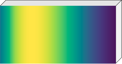\n\n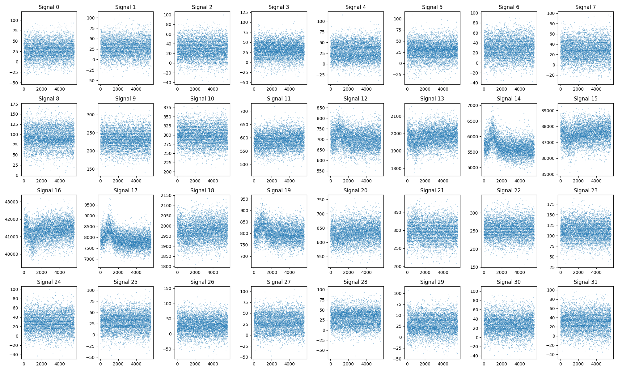\n\n## Initial Dip Estimation for Each Wavelength\n\n### Identifying the Transit Interval\n\nFor identifying the time location of the transit, the wavelength-averaged signal was used. After estimating the approximate time position using a rule-based algorithm, the exact time was identified with a fitting algorithm.\n\n### Gain Drift\n\nGain drift refers to the variation in the detector's gain over time and across different wavelengths. These drifts can introduce systematic errors in the observed signal and must be corrected to accurately estimate the transit dip.\n\nExoSim2 models the gain drift as:\n\n$$\n(1 + f(t) \\cdot g(\\lambda))\n$$\n\nwhere \\\\( f(t) \\\\) and \\\\( g(\\lambda) \\\\) are polynomial functions.\n\nIt is notable that the final function form is different from a two-variable polynomial \\\\( h(t, \\lambda) \\\\), because while the wavelength and time components can be separated in the former, they cannot in the latter.\n\nBy using this functional form directly in the fitting described below, we were able to achieve high performance in the dip estimation.\n\n### Dip Estimation with Gain Drift Fitting\n\nThe function used for fitting is as follows:\n\n$$\ny_{\\text{pred}} = I(\\lambda) \\times \\text{Box}(\\lambda) \\times (1 + f(t) \\cdot g(\\lambda))\n$$\n\nwhere \\\\( I(\\lambda) \\\\) is the spectrum of the star, and \\\\( \\text{Box}(\\lambda) \\\\) describes the dip; it is 1 outside the transit and \\\\( 1 - d_\\lambda \\\\) inside the transit.\n\nThe number of fitting parameters are as follows:\n\n- \\\\( f(t) \\\\): 5 parameters\n- \\\\( g(\\lambda) \\\\): 5 parameters\n\nIt is worth mentioning that the optimal \\\\( I(\\lambda) \\\\) and the optimal dip used in \\\\( \\text{Box}(\\lambda) \\\\), which minimize the mean squared error, can be found analytically if the other parameters are fixed, and they don't need to be considered by the fitting algorithm.\n\nTo stabilize the fitting process, a two-stage fitting was used. In the first stage, \\\\( I(\\lambda) \\\\) was directly estimated from the raw signal with temporal averaging and fixed during the fitting. In the second stage, \\\\( I(\\lambda) \\\\) was not fixed and was set optimally for each step during the fitting, while for the fitting parameters, the result from the first stage was used as the initial parameter. The error for each data point used in the fitting was estimated from the variation of the signal at each wavelength.\n\n### Dip Error Estimation with Bootstrapping\n\nThe errors in the dip estimation at each wavelength differ due to the varying signal-to-noise ratios associated with each wavelength. [Bootstrapping](https://en.wikipedia.org/wiki/Bootstrapping_(statistics)) was used to overcome this problem and to estimate the dip error of each wavelength.\n\nFurther details are available in our code.\n\n## Dip Estimation Considering Wavelength Correlations\n\nThree models were used: Gaussian Process Regression, AutoEncoder, and Non-negative Matrix Factorization (NMF). They were ensembled with the ratio 6:2:2.\n\n### Gaussian Process Regression\n\nNothing fancy, unlike the second-place solution.\n\nA simple kernel composed of RBF and Matern kernels was employed, and the errors calculated by bootstrapping were passed to `sklearn.gaussian_process.GaussianProcessRegressor` so that the model can consider the uncertainty of each data point.\n\n### AutoEncoder\n\nWe applied an autoencoder to capture relationships in the data.\n\nUnlike PCA, which captures linear relationships, autoencoders can model more complex and nonlinear patterns.\n\nAlso, we expected that by training the model with MSE loss, the autoencoder model could take noise into account and recover the \"optimal\" spectrum.\n\nImportant points were to normalize the data for each exoplanet and to take the moving median of the dip spectrum to smooth the input dip spectrum.\n\nThe model we used is as below, with 4 nodes in the hidden layer:\n\n```python\ninput_data = Input(shape=(input_dim,))\nencoded = Dense(encoding_dim, activation='relu')(input_data)\ndecoded = Dense(input_dim, activation='linear')(encoded)\n\nautoencoder = Model(input_data, decoded)\n```\n\n### NMF\n\nVery similar to the autoencoder, but we added it to enhance the diversity.\n\nUnlike with the autoencoder, the number of ranks was set to 5 for NMF.\n\n### Spectral Components Identified by NMF\n\nThe plot below shows the identified spectral components by NMF for the training data.\n\nIt can be seen that the main contributing gases of each component are:\n\n- **Component 1**: CO₂\n- **Component 2**: CH₄\n- **Component 3**: H₂O\n\nThis signifies NMF's ability to consider the correlation of the spectrum unsupervised.\n\n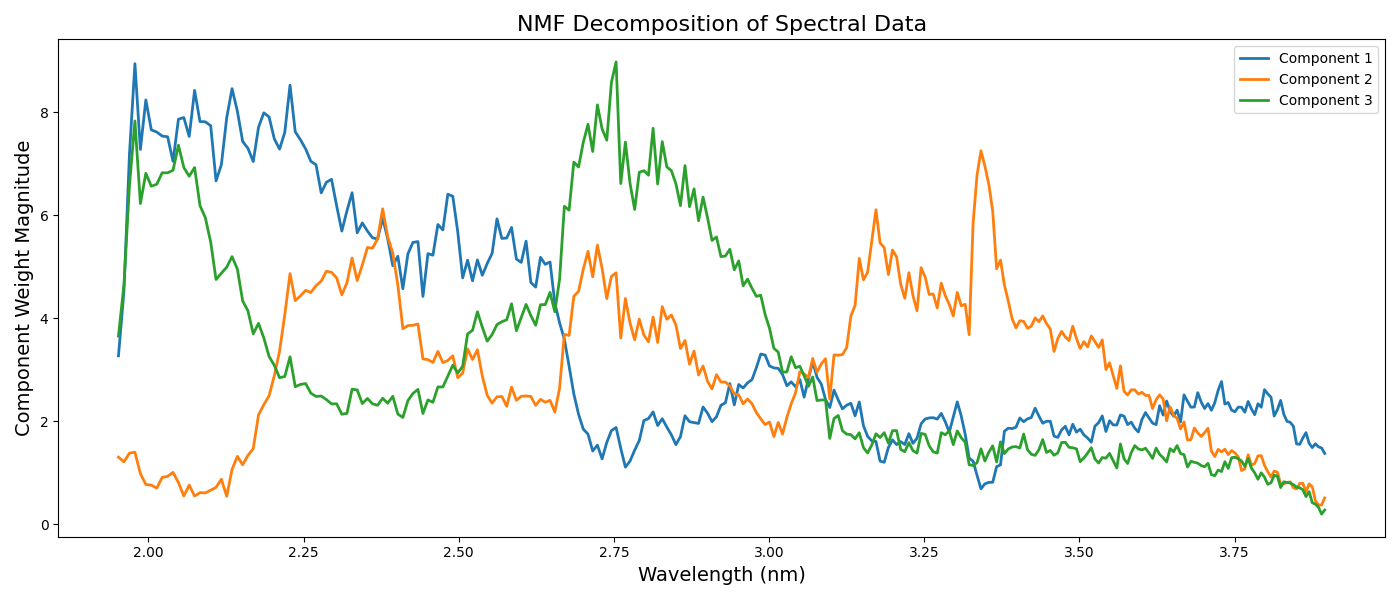\n\n### Sigma\n\nWe took the weighted average of the following components:\n\n1. **Constant value** (planet and wavelength independent)\n2. **Standard deviation of the smoothed predicted dip spectrum** (planet dependent, wavelength independent)\n3. **Uncertainty predicted by Gaussian Process Regression** (planet and wavelength dependent)\n\nThe constant value played an important role in cases where the dip spectrum was almost constant but had some bias.\n\n## The Contribution of Each Component\n\nSince our solution incorporates a variety of ideas, we examined the contributions for those that seem important with late submissions.\n\n| Method | Public | Private | Public Loss | Private Loss |\n|------------------------------------------------------------------|-------------|-------------|------------------|------------------|\n| **Final Submission** | 0.7330321 | 0.7420624 | 0.0000000 | 0.0000000 |\n| Only Gaussian Process Regression | 0.7221480 | 0.7343485 | -0.0108841 | -0.0077139 |\n| Only AutoEncoder | 0.7078056 | 0.7181137 | -0.0252265 | -0.0239487 |\n| Only NMF | 0.7017943 | 0.7122631 | -0.0312378 | -0.0297993 |\n| With Hot Pixel Processing | 0.7021653 | 0.7224989 | -0.0308668 | -0.0195635 |\n| Without Foreground ProcessingCongratulations on your win! It seems I didn't approach the competition enough as 'reproduce the synthetic data generation'. Nonetheless you also seem to have done a better job of breaking down the spectra than my simple PCA, which I expect could also benefit the final mission.
\nI'll also have to try a submission with the hot pixel processing disabled. This would be a bit disappointing if it matters much, since there were very few hot pixels in the training set (and so I never gave it much consideration).
", "rawMarkdown": "Congratulations on your win! It seems I didn't approach the competition enough as 'reproduce the synthetic data generation'. Nonetheless you also seem to have done a better job of breaking down the spectra than my simple PCA, which I expect could also benefit the final mission.\n\nI'll also have to try a submission with the hot pixel processing disabled. This would be a bit disappointing if it matters much, since there were very few hot pixels in the training set (and so I never gave it much consideration).", "votes": 6, "replies": [ { "id": 3036370, "postDate": "2024-11-04T13:54:14.670Z", "content": "I'm eager to see if your score jump to over 0.76 without the hot pixels, this would be amazing
", "rawMarkdown": "I'm eager to see if your score jump to over 0.76 without the hot pixels, this would be amazing", "votes": 2 }, { "id": 3036941, "postDate": "2024-11-05T04:45:19.040Z", "content": "I tested this and did not see an improvement by disabling the hot pixel filter. @cnumber , @daiwakun , do you apply any method to deal with invalid data? If not that might explain the difference. It's rather critical to deal with invalids, because jitter is only compensated when all rows are summed (as Jun Koda explains above). In fact you might gain more from some inpainting since it would also deal with dead pixels.
", "rawMarkdown": "I tested this and did not see an improvement by disabling the hot pixel filter. @cnumber , @daiwakun , do you apply any method to deal with invalid data? If not that might explain the difference. It's rather critical to deal with invalids, because jitter is only compensated when all rows are summed (as Jun Koda explains above). In fact you might gain more from some inpainting since it would also deal with dead pixels.", "votes": 3 }, { "id": 3037058, "postDate": "2024-11-05T09:40:28.540Z", "content": "For the dead pixels, and originally hot pixels, we didn't do anything special. Just a simple np.nanmean over the x-axis to get the signal for every wavelength. We also agree that the PSF distortion over time and the xy-axis jitter (as @junkoda pointed out) were the reasons why the hot pixel process hurt our score so much.
\nWe saw that your code interpolates nan pixels with adjacent pixels, and are assuming that maybe this is the reason why you didn't gain from deleting the hot pixel process.
", "rawMarkdown": "For the dead pixels, and originally hot pixels, we didn't do anything special. Just a simple np.nanmean over the x-axis to get the signal for every wavelength. We also agree that the PSF distortion over time and the xy-axis jitter (as @junkoda pointed out) were the reasons why the hot pixel process hurt our score so much.\n\nWe saw that your code interpolates nan pixels with adjacent pixels, and are assuming that maybe this is the reason why you didn't gain from deleting the hot pixel process.", "votes": 1, "replies": [ { "id": 3037059, "postDate": "2024-11-05T09:45:02.130Z", "content": "Why would interpolating dead affect the hot pixels? They are s separated iirc
", "rawMarkdown": "Why would interpolating dead affect the hot pixels? They are s separated iirc" }, { "id": 3037158, "postDate": "2024-11-05T12:27:24.707Z", "content": "I interpolate both dead and hot pixels.
", "rawMarkdown": "I interpolate both dead and hot pixels.", "votes": 1 }, { "id": 3037276, "postDate": "2024-11-05T14:55:01.933Z", "content": "We were curious of the impact of the interpolation on the score, so we added @jeroencottaar's interpolation code to our submission, and to our surprise found out that the interpolation had a huge impact on our score.
\n| Submission | \nPublic | \nPrivate | \n
|---|---|---|
| Without hot pixel process | \n0.7399976 | \n0.7450662 | \n
| With hot pixel process | \n0.73814190 | \n0.7448809 | \n
Nice! So hot pixels interpolation is the way
", "rawMarkdown": "Nice! So hot pixels interpolation is the way" } ] } ] }, { "id": 3036704, "postDate": "2024-11-04T20:39:59.737Z", "content": "I felt the dark current correction is too small (and speculated if the time 0.45 or 0.1 factor is really correct), so it makes scenes that keeping hot pixel is harmless and disadvantage in noise cancelling can be worse (but I didn't try).
\nThe PSF (point spread function) noise is highly correlated among spatial channels and the error is much less for the sum over 32 channels; not just 1/sqrt(N) reduction but noise is cancelling each other. I guessed this is subpixel pointing error - the star moves a little randomly during timestep so each spacial channel get a little different light but total is the same; or maybe the light get distorted for other reasons among pixels but within 32 channels. And the error cancellation become imperfect when pixel is removed, so not removing can be a benefit.
\nDo you only disable the hot pixels from dark current and keep the dead pixel mask? I think the Auto Encoder is great for learning the correlated error and compensate for the masked signal.
\nCongratulations for the 1st place!!!
", "rawMarkdown": "I felt the dark current correction is too small (and speculated if the time 0.45 or 0.1 factor is really correct), so it makes scenes that keeping hot pixel is harmless and disadvantage in noise cancelling can be worse (but I didn't try).\n\nThe PSF (point spread function) noise is highly correlated among spatial channels and the error is much less for the sum over 32 channels; not just 1/sqrt(N) reduction but noise is cancelling each other. I guessed this is subpixel pointing error - the star moves a little randomly during timestep so each spacial channel get a little different light but total is the same; or maybe the light get distorted for other reasons among pixels but within 32 channels. And the error cancellation become imperfect when pixel is removed, so not removing can be a benefit.\n\nDo you only disable the hot pixels from dark current and keep the dead pixel mask? I think the Auto Encoder is great for learning the correlated error and compensate for the masked signal.\n\nCongratulations for the 1st place!!!", "votes": 1, "replies": [ { "id": 3037052, "postDate": "2024-11-05T09:23:55.470Z", "content": "Thanks!
\n\n", "rawMarkdown": "Thanks!\n\n>Do you only disable the hot pixels from dark current and keep the dead pixel mask? \nYes. We believe that the process of the dead pixel mask is reasonable, and it was only the hot pixel mask that was doing the wrong things.", "votes": 1 } ] }, { "id": 3036376, "postDate": "2024-11-04T14:03:06.403Z", "content": "Do you only disable the hot pixels from dark current and keep the dead pixel mask?
\n
\n Yes. We believe that the process of the dead pixel mask is reasonable, and it was only the hot pixel mask that was doing the wrong things.
The link to the notebook the not work
", "rawMarkdown": "The link to the notebook the not work", "votes": 1, "replies": [ { "id": 3036377, "postDate": "2024-11-04T14:04:22.730Z", "content": "Sorry, forgot to make it public.
\nHope it works now!
Thank you. Congratz on winning; outstanding work.
", "rawMarkdown": "Thank you. Congratz on winning; outstanding work." }, { "id": 3036382, "postDate": "2024-11-04T14:11:53.547Z", "content": "I see 'private datasource' attached to your notebook, are they needed for it to run? If so, please public them too…
", "rawMarkdown": "I see 'private datasource' attached to your notebook, are they needed for it to run? If so, please public them too..." }, { "id": 3036386, "postDate": "2024-11-04T14:17:58.943Z", "content": "It's for installing astropy (and taurex_cuda), so you won't need it if you pip install it like this.
\nhttps://www.kaggle.com/discussions/product-feedback/532336
It was after attaching the datasource that I realised Kaggle had introduced this nice feature :(
", "rawMarkdown": "It's for installing astropy (and taurex_cuda), so you won't need it if you pip install it like this.\nhttps://www.kaggle.com/discussions/product-feedback/532336\n\nIt was after attaching the datasource that I realised Kaggle had introduced this nice feature :(", "votes": 1 } ] } ] }, { "id": 3036369, "postDate": "2024-11-04T13:52:53.213Z", "rawMarkdown": "", "isDeleted": true } ], "comments": [ { "id": 3036357, "author_name": "Jeroen Cottaar", "author_url": "", "post_date": "2024-11-04T13:44:31.620000", "content": "Congratulations on your win! It seems I didn't approach the competition enough as 'reproduce the synthetic data generation'. Nonetheless you also seem to have done a better job of breaking down the spectra than my simple PCA, which I expect could also benefit the final mission.
\nI'll also have to try a submission with the hot pixel processing disabled. This would be a bit disappointing if it matters much, since there were very few hot pixels in the training set (and so I never gave it much consideration).
", "votes": 6, "replies": [ { "id": 3036370, "author_name": "greySnow", "author_url": "", "post_date": "2024-11-04T13:54:14.670000", "content": "I'm eager to see if your score jump to over 0.76 without the hot pixels, this would be amazing
", "votes": 2, "replies": [] }, { "id": 3036941, "author_name": "Jeroen Cottaar", "author_url": "", "post_date": "2024-11-05T04:45:19.040000", "content": "I tested this and did not see an improvement by disabling the hot pixel filter. @cnumber , @daiwakun , do you apply any method to deal with invalid data? If not that might explain the difference. It's rather critical to deal with invalids, because jitter is only compensated when all rows are summed (as Jun Koda explains above). In fact you might gain more from some inpainting since it would also deal with dead pixels.
", "votes": 3, "replies": [] }, { "id": 3037058, "author_name": "c-number", "author_url": "", "post_date": "2024-11-05T09:40:28.540000", "content": "For the dead pixels, and originally hot pixels, we didn't do anything special. Just a simple np.nanmean over the x-axis to get the signal for every wavelength. We also agree that the PSF distortion over time and the xy-axis jitter (as @junkoda pointed out) were the reasons why the hot pixel process hurt our score so much.
\nWe saw that your code interpolates nan pixels with adjacent pixels, and are assuming that maybe this is the reason why you didn't gain from deleting the hot pixel process.
", "votes": 1, "replies": [ { "id": 3037059, "author_name": "greySnow", "author_url": "", "post_date": "2024-11-05T09:45:02.130000", "content": "Why would interpolating dead affect the hot pixels? They are s separated iirc
", "votes": 0, "replies": [] }, { "id": 3037158, "author_name": "Jeroen Cottaar", "author_url": "", "post_date": "2024-11-05T12:27:24.707000", "content": "I interpolate both dead and hot pixels.
", "votes": 1, "replies": [] }, { "id": 3037276, "author_name": "c-number", "author_url": "", "post_date": "2024-11-05T14:55:01.933000", "content": "We were curious of the impact of the interpolation on the score, so we added @jeroencottaar's interpolation code to our submission, and to our surprise found out that the interpolation had a huge impact on our score.
\n| Submission | \nPublic | \nPrivate | \n
|---|---|---|
| Without hot pixel process | \n0.7399976 | \n0.7450662 | \n
| With hot pixel process | \n0.73814190 | \n0.7448809 | \n
Nice! So hot pixels interpolation is the way
", "votes": 0, "replies": [] } ] } ] }, { "id": 3036704, "author_name": "🐢 Jun Koda", "author_url": "", "post_date": "2024-11-04T20:39:59.737000", "content": "I felt the dark current correction is too small (and speculated if the time 0.45 or 0.1 factor is really correct), so it makes scenes that keeping hot pixel is harmless and disadvantage in noise cancelling can be worse (but I didn't try).
\nThe PSF (point spread function) noise is highly correlated among spatial channels and the error is much less for the sum over 32 channels; not just 1/sqrt(N) reduction but noise is cancelling each other. I guessed this is subpixel pointing error - the star moves a little randomly during timestep so each spacial channel get a little different light but total is the same; or maybe the light get distorted for other reasons among pixels but within 32 channels. And the error cancellation become imperfect when pixel is removed, so not removing can be a benefit.
\nDo you only disable the hot pixels from dark current and keep the dead pixel mask? I think the Auto Encoder is great for learning the correlated error and compensate for the masked signal.
\nCongratulations for the 1st place!!!
", "votes": 1, "replies": [ { "id": 3037052, "author_name": "c-number", "author_url": "", "post_date": "2024-11-05T09:23:55.470000", "content": "Thanks!
\n\n", "votes": 1, "replies": [] } ] }, { "id": 3036376, "author_name": "greySnow", "author_url": "", "post_date": "2024-11-04T14:03:06.403000", "content": "Do you only disable the hot pixels from dark current and keep the dead pixel mask?
\n
\n Yes. We believe that the process of the dead pixel mask is reasonable, and it was only the hot pixel mask that was doing the wrong things.
The link to the notebook the not work
", "votes": 1, "replies": [ { "id": 3036377, "author_name": "c-number", "author_url": "", "post_date": "2024-11-04T14:04:22.730000", "content": "Sorry, forgot to make it public.
\nHope it works now!
Thank you. Congratz on winning; outstanding work.
", "votes": 0, "replies": [] }, { "id": 3036382, "author_name": "greySnow", "author_url": "", "post_date": "2024-11-04T14:11:53.547000", "content": "I see 'private datasource' attached to your notebook, are they needed for it to run? If so, please public them too…
", "votes": 0, "replies": [] }, { "id": 3036386, "author_name": "c-number", "author_url": "", "post_date": "2024-11-04T14:17:58.943000", "content": "It's for installing astropy (and taurex_cuda), so you won't need it if you pip install it like this.
\nhttps://www.kaggle.com/discussions/product-feedback/532336
It was after attaching the datasource that I realised Kaggle had introduced this nice feature :(
", "votes": 1, "replies": [] } ] } ] }, { "id": 3036369, "author_name": "", "author_url": "", "post_date": "2024-11-04T13:52:53.213000", "content": "", "votes": 0, "replies": [] } ], "raw_markdown_by_id": { "3036336": "[link to notebook](https://www.kaggle.com/code/cnumber/neurips-ariel-data-challenge-2024-final-submission)\n\n# Introduction\n\nWe ( @daiwakun and @cnumber) would like to thank the organizers for hosting this fascinating competition, especially @gordonyip and @lorenzomugnai, who worked tirelessly so that competitors could focus on the more \"interesting\" parts.\n\nAlso, a huge applause to @jeroencottaar for maintaining first place for almost the entire duration of the competition. Although we managed to grab victory at the end of the race, we are confident that we would have lost had the competition period been one day shorter or one day longer.\n\nMany ideas in our solution were found during a deep examination of the ExoSim2 and TauREx3 code used for data generation, including gain drift fitting and foreground processing. Although we didn't (or couldn't) find any leaks, we have to admit that our solution somewhat \"hacks\" the simulator. Nevertheless, we hope the hosts can make use of some aspects of our solution, and hopefully, it would be useful for the actual data.\n\nFor those who are curious about our significant score improvement during the last two days of the competition, we have decided to present what was going on in our team in [another post](https://www.kaggle.com/competitions/ariel-data-challenge-2024/discussion/544316)\n\n# Solution\n\n## Signal Preprocessing\n\nOnly the AIRS-CH0 channel was used because our solution heavily relies on the correlation between adjacent wavelengths, and also because we were unsure how to effectively utilize the FGS1 channel data due to issues with its distorted and fluctuating point spread function.\n\nThe public notebook (we wanted to put a link, but we couldn't find the notebook we used) was used with the following changes:\n\n1. **Disabling Hot Pixel Processing**: This led to a significant jump on the leaderboard. We assume that the hot pixel processing leads to unwanted information loss of the pixels in the middle of the sensor, making it almost impossible to correct the noise introduced by the time-dependent PSF distortion (see image below). Perhaps it is the sigma clip algorithm that is doing the wrong thing and that there exist algorithms that can handle hot pixels properly, but we weren't able to find them.\n\n2. **Foreground Processing**: Some teams have noticed that multiplying the final spectrum by a coefficient around 1.006~1.008 gives a huge boost. This is because a foreground is added to the signal during the ExoSim2 simulation [link to GitHub]. The correct way to handle this is to estimate the wavelength-dependent foreground signal and to subtract it from the signal in the central region. In our solution, we decided to estimate the foreground signal with the regions `[0:8]` and `[24:32]`, and subtracted it from the central region `[8:24]`. The effect of considering the foreground properly can be seen in [this discussion post](https://www.kaggle.com/competitions/ariel-data-challenge-2024/discussion/543853#3034987).\n\n\n\n\n\n## Initial Dip Estimation for Each Wavelength\n\n### Identifying the Transit Interval\n\nFor identifying the time location of the transit, the wavelength-averaged signal was used. After estimating the approximate time position using a rule-based algorithm, the exact time was identified with a fitting algorithm.\n\n### Gain Drift\n\nGain drift refers to the variation in the detector's gain over time and across different wavelengths. These drifts can introduce systematic errors in the observed signal and must be corrected to accurately estimate the transit dip.\n\nExoSim2 models the gain drift as:\n\n$$\n(1 + f(t) \\cdot g(\\lambda))\n$$\n\nwhere \\\\( f(t) \\\\) and \\\\( g(\\lambda) \\\\) are polynomial functions.\n\nIt is notable that the final function form is different from a two-variable polynomial \\\\( h(t, \\lambda) \\\\), because while the wavelength and time components can be separated in the former, they cannot in the latter.\n\nBy using this functional form directly in the fitting described below, we were able to achieve high performance in the dip estimation.\n\n### Dip Estimation with Gain Drift Fitting\n\nThe function used for fitting is as follows:\n\n$$\ny_{\\text{pred}} = I(\\lambda) \\times \\text{Box}(\\lambda) \\times (1 + f(t) \\cdot g(\\lambda))\n$$\n\nwhere \\\\( I(\\lambda) \\\\) is the spectrum of the star, and \\\\( \\text{Box}(\\lambda) \\\\) describes the dip; it is 1 outside the transit and \\\\( 1 - d_\\lambda \\\\) inside the transit.\n\nThe number of fitting parameters are as follows:\n\n- \\\\( f(t) \\\\): 5 parameters\n- \\\\( g(\\lambda) \\\\): 5 parameters\n\nIt is worth mentioning that the optimal \\\\( I(\\lambda) \\\\) and the optimal dip used in \\\\( \\text{Box}(\\lambda) \\\\), which minimize the mean squared error, can be found analytically if the other parameters are fixed, and they don't need to be considered by the fitting algorithm.\n\nTo stabilize the fitting process, a two-stage fitting was used. In the first stage, \\\\( I(\\lambda) \\\\) was directly estimated from the raw signal with temporal averaging and fixed during the fitting. In the second stage, \\\\( I(\\lambda) \\\\) was not fixed and was set optimally for each step during the fitting, while for the fitting parameters, the result from the first stage was used as the initial parameter. The error for each data point used in the fitting was estimated from the variation of the signal at each wavelength.\n\n### Dip Error Estimation with Bootstrapping\n\nThe errors in the dip estimation at each wavelength differ due to the varying signal-to-noise ratios associated with each wavelength. [Bootstrapping](https://en.wikipedia.org/wiki/Bootstrapping_(statistics)) was used to overcome this problem and to estimate the dip error of each wavelength.\n\nFurther details are available in our code.\n\n## Dip Estimation Considering Wavelength Correlations\n\nThree models were used: Gaussian Process Regression, AutoEncoder, and Non-negative Matrix Factorization (NMF). They were ensembled with the ratio 6:2:2.\n\n### Gaussian Process Regression\n\nNothing fancy, unlike the second-place solution.\n\nA simple kernel composed of RBF and Matern kernels was employed, and the errors calculated by bootstrapping were passed to `sklearn.gaussian_process.GaussianProcessRegressor` so that the model can consider the uncertainty of each data point.\n\n### AutoEncoder\n\nWe applied an autoencoder to capture relationships in the data.\n\nUnlike PCA, which captures linear relationships, autoencoders can model more complex and nonlinear patterns.\n\nAlso, we expected that by training the model with MSE loss, the autoencoder model could take noise into account and recover the \"optimal\" spectrum.\n\nImportant points were to normalize the data for each exoplanet and to take the moving median of the dip spectrum to smooth the input dip spectrum.\n\nThe model we used is as below, with 4 nodes in the hidden layer:\n\n```python\ninput_data = Input(shape=(input_dim,))\nencoded = Dense(encoding_dim, activation='relu')(input_data)\ndecoded = Dense(input_dim, activation='linear')(encoded)\n\nautoencoder = Model(input_data, decoded)\n```\n\n### NMF\n\nVery similar to the autoencoder, but we added it to enhance the diversity.\n\nUnlike with the autoencoder, the number of ranks was set to 5 for NMF.\n\n### Spectral Components Identified by NMF\n\nThe plot below shows the identified spectral components by NMF for the training data.\n\nIt can be seen that the main contributing gases of each component are:\n\n- **Component 1**: CO₂\n- **Component 2**: CH₄\n- **Component 3**: H₂O\n\nThis signifies NMF's ability to consider the correlation of the spectrum unsupervised.\n\n\n\n### Sigma\n\nWe took the weighted average of the following components:\n\n1. **Constant value** (planet and wavelength independent)\n2. **Standard deviation of the smoothed predicted dip spectrum** (planet dependent, wavelength independent)\n3. **Uncertainty predicted by Gaussian Process Regression** (planet and wavelength dependent)\n\nThe constant value played an important role in cases where the dip spectrum was almost constant but had some bias.\n\n## The Contribution of Each Component\n\nSince our solution incorporates a variety of ideas, we examined the contributions for those that seem important with late submissions.\n\n| Method | Public | Private | Public Loss | Private Loss |\n|------------------------------------------------------------------|-------------|-------------|------------------|------------------|\n| **Final Submission** | 0.7330321 | 0.7420624 | 0.0000000 | 0.0000000 |\n| Only Gaussian Process Regression | 0.7221480 | 0.7343485 | -0.0108841 | -0.0077139 |\n| Only AutoEncoder | 0.7078056 | 0.7181137 | -0.0252265 | -0.0239487 |\n| Only NMF | 0.7017943 | 0.7122631 | -0.0312378 | -0.0297993 |\n| With Hot Pixel Processing | 0.7021653 | 0.7224989 | -0.0308668 | -0.0195635 |\n| Without Foreground Processing