
I'd first like to thank the organizers for putting on such an interesting competition. They deserve credit both for their scientific rigor and for the intricate puzzles they used to generate the data—some of which I still haven't managed to solve.
\nThis solution presents a comprehensive, three-stage pipeline designed to extract high-fidelity transmission spectra from the FGS1 and AIR-CH0 Ariel instrument data. The approach combines physics-based modeling with a machine learning-inspired post-processing framework to tackle the key challenges of instrumental systematics and uncertainty estimation.
\nStage 1: GPU-Accelerated Preprocessing. Raw sensor data is converted into clean, calibrated light curves using a CuPy-based pipeline. This stage handles standard instrumental corrections, including non-linearity, dark current, flat-fielding, and jitter, all performed efficiently on the GPU.
Stage 2: Hierarchical Transit Fitting. I use the batman transit modeling library and the iminuit optimizer to perform a multi-step fit. A robust global model is first fit to the combined FGS and AIRS light curves to constrain key orbital parameters. This is followed by a 2D drift correction and a wavelength-by-wavelength fit to extract the initial transmission spectrum.
Stage 3: Cross-Validated Post-Processing Ensemble. The initial spectra are refined using an ensemble of models trained with Grouped K-Fold Cross-Validation. This final stage blends a PCA-regularized signal with a smoothed signal and employs a parameterized model to predict the final uncertainties (sigmas), optimizing all parameters directly against the competition score.
This multi-stage design ensures that physical constraints are respected in the initial fit, while the final model has the flexibility to learn and correct for residual systematic errors and produce well-calibrated uncertainties.
\nThe first step in the pipeline is to transform the raw sensor readouts into scientifically useful light curves. This entire process is executed on the GPU using CuPy for maximum efficiency.
\nKey Preprocessing Steps:
\n• Initial Calibrations: The pipeline begins by applying standard instrumental corrections. This includes an ADC correction for gain and offset, a 5th-degree polynomial correction for detector non-linearity (apply_linear_corr_fast), and subtraction of a scaled master dark frame (clean_dark).
\n• Flat-Fielding & Masking: A master flat frame is applied to correct for pixel-to-pixel sensitivity variations. Pixels identified as \"hot\" (via sigma-clipping the dark frame) or \"dead\" are masked.
\n• Jitter Correction: For the FGS1 sensor, we apply a center-of-mass regression to correct for flux variations caused by image motion on the detector. The flux is de-correlated from the normalized X and Y positions of the stellar image. While a PCA-based jitter correction method was developed for the AIRS sensor, it was found to be less effective and is disabled in the final pipeline.
\n
• Signal Extraction & Cleaning:
\n
• Binning: To improve the signal-to-noise ratio, the final time series for both instruments are binned by averaging consecutive frames.
\nWith clean light curves for both instruments, we extract the initial transmission spectrum. This process is parallelized using pqdm to efficiently process all observations.
\nHierarchical Fitting Strategy:
\n1. Global Combined Fit: We first fit the FGS light curve and the wavelength-averaged AIRS light curve simultaneously using fit_combined_curves. This crucial step provides robust constraints on the shared physical parameters of the system (e.g., orbital period per, inclination inc, transit time t0), which are initialized from the provided star_info.csv file. The transit is modeled using batman, asuming a quadratic limb darkening model, using 2 parameters, and instrumental trends are modeled with a polynomial baseline in time.
\n
2. Refined Fit & Drift Correction: The results from the first fit are used to initialize a second, refined fit on normalized data. Subsequently, a 2D instrumental drift model is fit to the out-of-transit portion of the AIRS data cube. This model (Drift class) consists of two 4th-order polynomials, one for the frequency and one for the temporal axis, and it corrects for slow-varying systematic patterns across the detector. The data cube is then divided by this drift model.
\n3. Wavelength-by-Wavelength Fit: The final step is to measure the transit depth in each individual wavelength channel of the drift-corrected AIRS data. The fit_w function iterates through the channels, fitting the data within a small moving window (deltaw=2) to boost signal-to-noise. In this fit, most orbital parameters are fixed to the values from the global fit, and only the transit depth (dipa) and baseline normalization (A0a) are allowed to vary.
\nThis process results in the \"raw\" spectrum and its associated uncertainties , which serve as the primary inputs for our final modeling stage.

The final stage of the solution is a post-processing model that refines the raw spectra and, critically, learns a robust model for the final uncertainties. This is where the bulk of the \"machine learning\" occurs.
\nModel Architecture (build_preds): The model generates a final prediction by blending two different representations of the raw spectrum (preds1):
\nPCA-Regularized Prediction (preds0): The raw spectrum undergoes a slope correction and is then projected onto a pre-defined PCA basis (components.npy). This de-noises the spectrum and imposes a strong regularization prior, capturing the most common modes of variation.
\nSmoothed Prediction (preds2): The raw AIRS spectrum is smoothed using a Savitzky-Golay filter to reduce high-frequency noise while preserving broader spectral features.
The final mean prediction is a weighted average of these two models: preds = app0 + (1-ap)preds2, where ap is a learned parameter.
\nSigma Model: Predicting accurate uncertainties is key to maximizing the competition score. I developed a complex, empirically-derived formula to model the final sigma for each data point. This formula combines multiple sources of uncertainty:
\nFinally ther is a sigma adjustment samples with very few or very many out-of-transit points, or very differnt dip por FGS1 and AIR-CH0
\nObjective: The free parameters of the model (ap, e1, e2, a1, a0, b0, ae, etc.) are optimized using iminuit to directly maximize the competition score.
\nCross-Validation: To build a robust model that generalizes well, we employ a 10-fold Grouped K-Fold Cross-Validation strategy, using planet_id to group the data. This ensures that all observations of a single planet are kept within the same fold, preventing data leakage.
\nCalibration: Within each fold, after the primary parameters are optimized, we calculate a wavelength-dependent calibration factor (alpha) that scales the predicted sigmas to best match the variance observed in the training data. This factor is then applied to the validation set predictions.
\nEnsembling: The final submission is generated by averaging the calibrated predictions and sigmas from the 10 models trained during the cross-validation process. This ensembling technique reduces variance and improves the final score.
\nThe entire training process, including the parallel optimization of each fold, is managed by the CV_model function in the model.py file.
\nIn the final weeks, I spent time trying to isolate the additive foreground noise in the AIRS data for each sample, which would have eliminated the need for the global factor and slope compensation. However, I was unable to find a way to de-correlate signal and noise. I observed a clear structure in the spectroscopic PSF, but all attempts to extract the noise yielded incorrect values that failed to compensate for the systematics.
\nThis solution demonstrates the power of a hybrid approach, blending physics-informed transit modeling with a flexible, data-driven post-processing framework. By first extracting a reasonable physical spectrum and then refining it with a model trained to optimize the specific competition metric, we can effectively correct for complex instrumental systematics and produce highly accurate, well-calibrated transmission spectra. The use of GPU acceleration, parallel processing, and a robust cross-validation scheme ensures that this complex pipeline remains computationally efficient and resistant to overfitting.
", "messages": [ { "id": 3294167, "postDate": "2025-09-25T13:59:48.953Z", "content": "I'd first like to thank the organizers for putting on such an interesting competition. They deserve credit both for their scientific rigor and for the intricate puzzles they used to generate the data—some of which I still haven't managed to solve.
\nThis solution presents a comprehensive, three-stage pipeline designed to extract high-fidelity transmission spectra from the FGS1 and AIR-CH0 Ariel instrument data. The approach combines physics-based modeling with a machine learning-inspired post-processing framework to tackle the key challenges of instrumental systematics and uncertainty estimation.
\nStage 1: GPU-Accelerated Preprocessing. Raw sensor data is converted into clean, calibrated light curves using a CuPy-based pipeline. This stage handles standard instrumental corrections, including non-linearity, dark current, flat-fielding, and jitter, all performed efficiently on the GPU.
Stage 2: Hierarchical Transit Fitting. I use the batman transit modeling library and the iminuit optimizer to perform a multi-step fit. A robust global model is first fit to the combined FGS and AIRS light curves to constrain key orbital parameters. This is followed by a 2D drift correction and a wavelength-by-wavelength fit to extract the initial transmission spectrum.
Stage 3: Cross-Validated Post-Processing Ensemble. The initial spectra are refined using an ensemble of models trained with Grouped K-Fold Cross-Validation. This final stage blends a PCA-regularized signal with a smoothed signal and employs a parameterized model to predict the final uncertainties (sigmas), optimizing all parameters directly against the competition score.
This multi-stage design ensures that physical constraints are respected in the initial fit, while the final model has the flexibility to learn and correct for residual systematic errors and produce well-calibrated uncertainties.
\nThe first step in the pipeline is to transform the raw sensor readouts into scientifically useful light curves. This entire process is executed on the GPU using CuPy for maximum efficiency.
\nKey Preprocessing Steps:
\n• Initial Calibrations: The pipeline begins by applying standard instrumental corrections. This includes an ADC correction for gain and offset, a 5th-degree polynomial correction for detector non-linearity (apply_linear_corr_fast), and subtraction of a scaled master dark frame (clean_dark).
\n• Flat-Fielding & Masking: A master flat frame is applied to correct for pixel-to-pixel sensitivity variations. Pixels identified as \"hot\" (via sigma-clipping the dark frame) or \"dead\" are masked.
\n• Jitter Correction: For the FGS1 sensor, we apply a center-of-mass regression to correct for flux variations caused by image motion on the detector. The flux is de-correlated from the normalized X and Y positions of the stellar image. While a PCA-based jitter correction method was developed for the AIRS sensor, it was found to be less effective and is disabled in the final pipeline.
\n
• Signal Extraction & Cleaning:
\n• Binning: To improve the signal-to-noise ratio, the final time series for both instruments are binned by averaging consecutive frames.
\nWith clean light curves for both instruments, we extract the initial transmission spectrum. This process is parallelized using pqdm to efficiently process all observations.
\nHierarchical Fitting Strategy:
\n1. Global Combined Fit: We first fit the FGS light curve and the wavelength-averaged AIRS light curve simultaneously using fit_combined_curves. This crucial step provides robust constraints on the shared physical parameters of the system (e.g., orbital period per, inclination inc, transit time t0), which are initialized from the provided star_info.csv file. The transit is modeled using batman, asuming a quadratic limb darkening model, using 2 parameters, and instrumental trends are modeled with a polynomial baseline in time.
\n
2. Refined Fit & Drift Correction: The results from the first fit are used to initialize a second, refined fit on normalized data. Subsequently, a 2D instrumental drift model is fit to the out-of-transit portion of the AIRS data cube. This model (Drift class) consists of two 4th-order polynomials, one for the frequency and one for the temporal axis, and it corrects for slow-varying systematic patterns across the detector. The data cube is then divided by this drift model.
\n3. Wavelength-by-Wavelength Fit: The final step is to measure the transit depth in each individual wavelength channel of the drift-corrected AIRS data. The fit_w function iterates through the channels, fitting the data within a small moving window (deltaw=2) to boost signal-to-noise. In this fit, most orbital parameters are fixed to the values from the global fit, and only the transit depth (dipa) and baseline normalization (A0a) are allowed to vary.
\nThis process results in the \"raw\" spectrum and its associated uncertainties , which serve as the primary inputs for our final modeling stage.
The final stage of the solution is a post-processing model that refines the raw spectra and, critically, learns a robust model for the final uncertainties. This is where the bulk of the \"machine learning\" occurs.
\nModel Architecture (build_preds): The model generates a final prediction by blending two different representations of the raw spectrum (preds1):
\nPCA-Regularized Prediction (preds0): The raw spectrum undergoes a slope correction and is then projected onto a pre-defined PCA basis (components.npy). This de-noises the spectrum and imposes a strong regularization prior, capturing the most common modes of variation.
\nSmoothed Prediction (preds2): The raw AIRS spectrum is smoothed using a Savitzky-Golay filter to reduce high-frequency noise while preserving broader spectral features.
The final mean prediction is a weighted average of these two models: preds = app0 + (1-ap)preds2, where ap is a learned parameter.
\nSigma Model: Predicting accurate uncertainties is key to maximizing the competition score. I developed a complex, empirically-derived formula to model the final sigma for each data point. This formula combines multiple sources of uncertainty:
\nFinally ther is a sigma adjustment samples with very few or very many out-of-transit points, or very differnt dip por FGS1 and AIR-CH0
\nObjective: The free parameters of the model (ap, e1, e2, a1, a0, b0, ae, etc.) are optimized using iminuit to directly maximize the competition score.
\nCross-Validation: To build a robust model that generalizes well, we employ a 10-fold Grouped K-Fold Cross-Validation strategy, using planet_id to group the data. This ensures that all observations of a single planet are kept within the same fold, preventing data leakage.
\nCalibration: Within each fold, after the primary parameters are optimized, we calculate a wavelength-dependent calibration factor (alpha) that scales the predicted sigmas to best match the variance observed in the training data. This factor is then applied to the validation set predictions.
\nEnsembling: The final submission is generated by averaging the calibrated predictions and sigmas from the 10 models trained during the cross-validation process. This ensembling technique reduces variance and improves the final score.
\nThe entire training process, including the parallel optimization of each fold, is managed by the CV_model function in the model.py file.
\nIn the final weeks, I spent time trying to isolate the additive foreground noise in the AIRS data for each sample, which would have eliminated the need for the global factor and slope compensation. However, I was unable to find a way to de-correlate signal and noise. I observed a clear structure in the spectroscopic PSF, but all attempts to extract the noise yielded incorrect values that failed to compensate for the systematics.
\nThis solution demonstrates the power of a hybrid approach, blending physics-informed transit modeling with a flexible, data-driven post-processing framework. By first extracting a reasonable physical spectrum and then refining it with a model trained to optimize the specific competition metric, we can effectively correct for complex instrumental systematics and produce highly accurate, well-calibrated transmission spectra. The use of GPU acceleration, parallel processing, and a robust cross-validation scheme ensures that this complex pipeline remains computationally efficient and resistant to overfitting.
", "rawMarkdown": "# Ariel 25 Challenge: A Three-Stage Pipeline for Robust Transmission Spectra\n\nI'd first like to thank the organizers for putting on such an interesting competition. They deserve credit both for their scientific rigor and for the intricate puzzles they used to generate the data—some of which I still haven't managed to solve.\n\n##1. Summary\n\nThis solution presents a comprehensive, three-stage pipeline designed to extract high-fidelity transmission spectra from the FGS1 and AIR-CH0 Ariel instrument data. The approach combines physics-based modeling with a machine learning-inspired post-processing framework to tackle the key challenges of instrumental systematics and uncertainty estimation.\n\n1. Stage 1: GPU-Accelerated Preprocessing. Raw sensor data is converted into clean, calibrated light curves using a CuPy-based pipeline. This stage handles standard instrumental corrections, including non-linearity, dark current, flat-fielding, and jitter, all performed efficiently on the GPU.\n\n2. Stage 2: Hierarchical Transit Fitting. I use the [**batman**](https://lkreidberg.github.io/batman/docs/html/index.html) transit modeling library and the [**iminuit**](https://scikit-hep.org/iminuit/) optimizer to perform a multi-step fit. A robust global model is first fit to the combined FGS and AIRS light curves to constrain key orbital parameters. This is followed by a 2D drift correction and a wavelength-by-wavelength fit to extract the initial transmission spectrum.\n\n3. Stage 3: Cross-Validated Post-Processing Ensemble. The initial spectra are refined using an ensemble of models trained with Grouped K-Fold Cross-Validation. This final stage blends a PCA-regularized signal with a smoothed signal and employs a parameterized model to predict the final uncertainties (sigmas), optimizing all parameters directly against the competition score.\n\n\nThis multi-stage design ensures that physical constraints are respected in the initial fit, while the final model has the flexibility to learn and correct for residual systematic errors and produce well-calibrated uncertainties.\n\n--------------------------------------------------------------------------------\n## 2. Methodology\n\n###Stage 1: Preprocessing Raw Data\nThe first step in the pipeline is to transform the raw sensor readouts into scientifically useful light curves. This entire process is executed on the GPU using CuPy for maximum efficiency.\n\nKey Preprocessing Steps:\n\n• Initial Calibrations: The pipeline begins by applying standard instrumental corrections. This includes an ADC correction for gain and offset, a 5th-degree polynomial correction for detector non-linearity (apply_linear_corr_fast), and subtraction of a scaled master dark frame (clean_dark).\n\n• Flat-Fielding & Masking: A master flat frame is applied to correct for pixel-to-pixel sensitivity variations. Pixels identified as \"hot\" (via sigma-clipping the dark frame) or \"dead\" are masked.\n\n• Jitter Correction: For the FGS1 sensor, we apply a center-of-mass regression to correct for flux variations caused by image motion on the detector. The flux is de-correlated from the normalized X and Y positions of the stellar image. While a PCA-based jitter correction method was developed for the AIRS sensor, it was found to be less effective and is disabled in the final pipeline.\n\n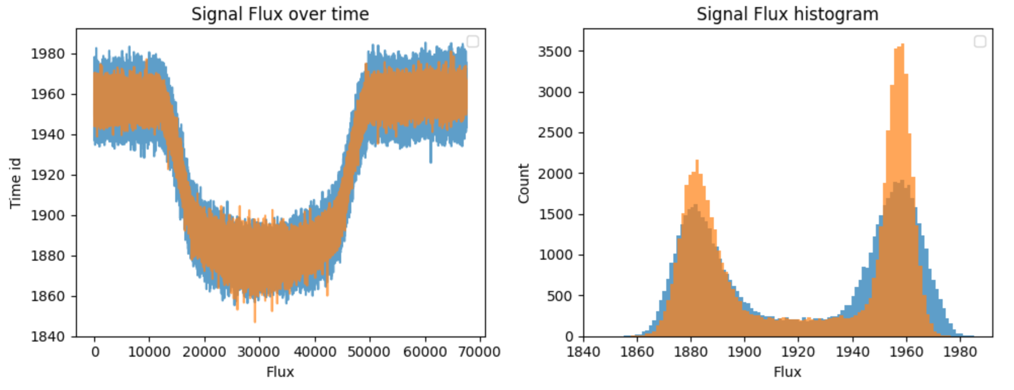\n\n\n\n• Signal Extraction & Cleaning:\n\n \n* For FGS1, the final flux is extracted using simple aperture photometry. PSF photometry gives lower SNR signals, probably due to the jitter.\n* For AIRS, the signal is extracted from the central detector region, and a background signal, calculated from the top and bottom edges of the detector, is subtracted. This is not optimal because the spectroscopy signal extends i a difractive way to the whole sensor, making dificult to identify the aditive frequency dependent background and making necessary a global scale factor and an spectrum slope correction in the post processing stage\n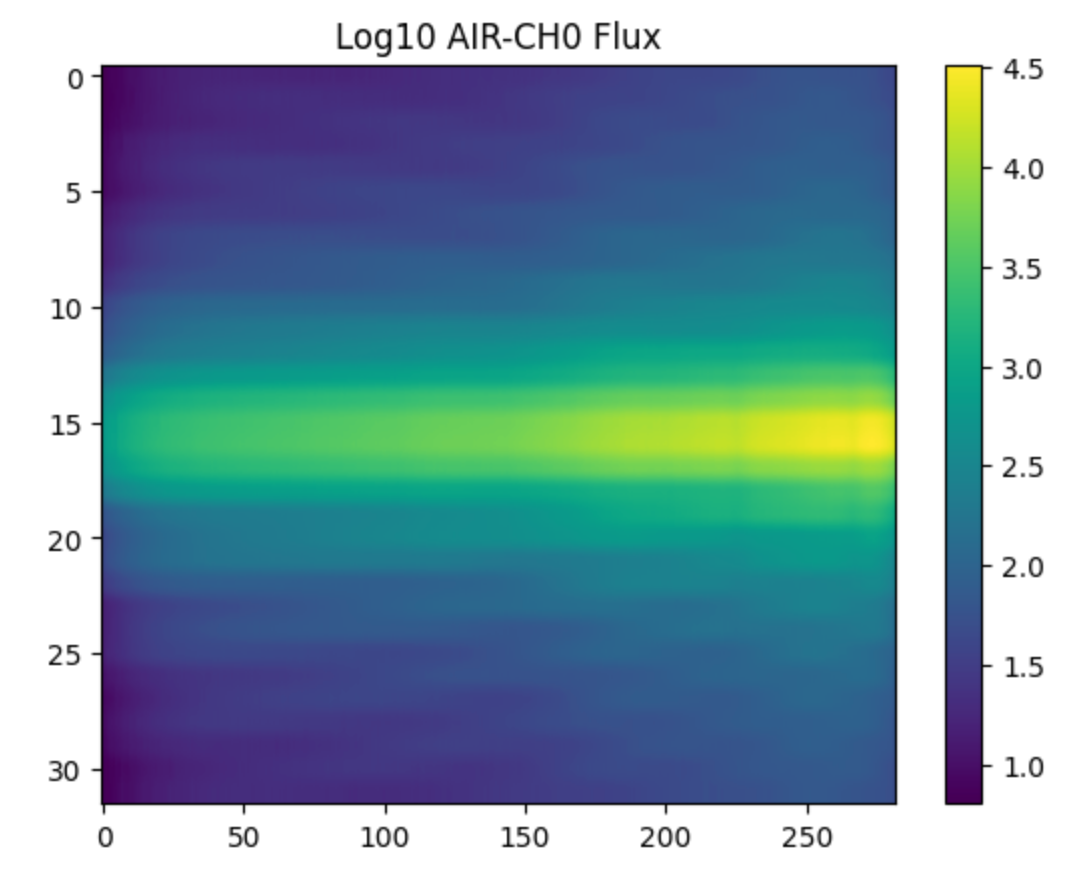\n* A spike-cleaning algorithm is applied to the final time series to remove cosmic ray hits by identifying and replacing outliers in the frame-to-frame difference.\n\n \n• Binning: To improve the signal-to-noise ratio, the final time series for both instruments are binned by averaging consecutive frames.\n\n###Stage 2: Physics-Based Spectral Fitting\n\nWith clean light curves for both instruments, we extract the initial transmission spectrum. This process is parallelized using pqdm to efficiently process all observations.\n\nHierarchical Fitting Strategy:\n\n**1. Global Combined Fit**: We first fit the FGS light curve and the wavelength-averaged AIRS light curve **simultaneously** using fit_combined_curves. This crucial step provides robust constraints on the shared physical parameters of the system (e.g., orbital period per, inclination inc, transit time t0), which are initialized from the provided star_info.csv file. The transit is modeled using batman, asuming a **quadratic limb darkening model**, using 2 parameters, and instrumental trends are modeled with a polynomial baseline in time.\n\n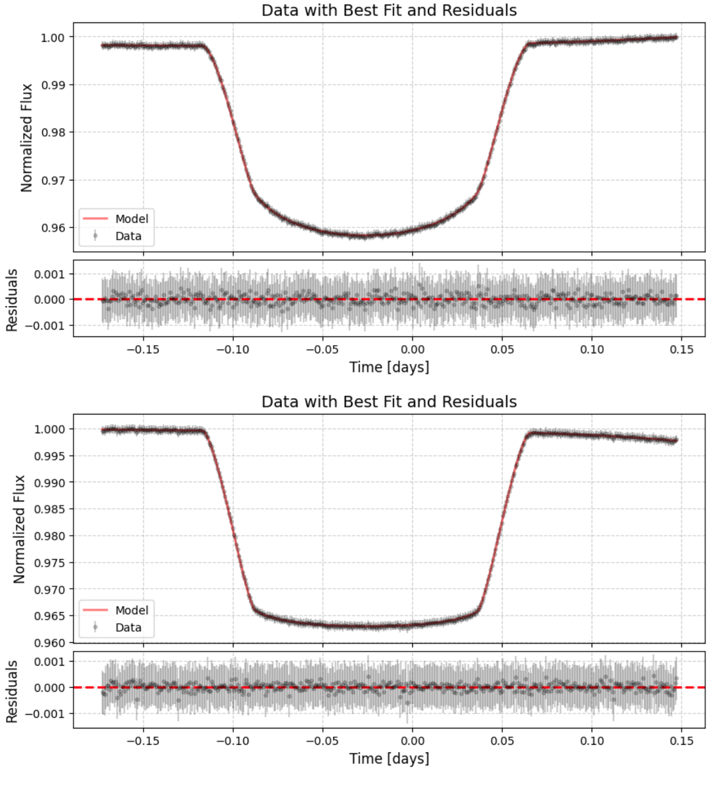\n\n**2. Refined Fit & Drift Correction**: The results from the first fit are used to initialize a second, refined fit on normalized data. Subsequently, a 2D instrumental drift model is fit to the out-of-transit portion of the AIRS data cube. This model (Drift class) consists of two 4th-order polynomials, one for the frequency and one for the temporal axis, and it corrects for slow-varying systematic patterns across the detector. The data cube is then divided by this drift model.\n**3. Wavelength-by-Wavelength Fit**: The final step is to measure the transit depth in each individual wavelength channel of the drift-corrected AIRS data. The fit_w function iterates through the channels, fitting the data within a small moving window (deltaw=2) to boost signal-to-noise. In this fit, most orbital parameters are fixed to the values from the global fit, and only the transit depth (dipa) and baseline normalization (A0a) are allowed to vary.\nThis process results in the \"raw\" spectrum and its associated uncertainties , which serve as the primary inputs for our final modeling stage.\n\n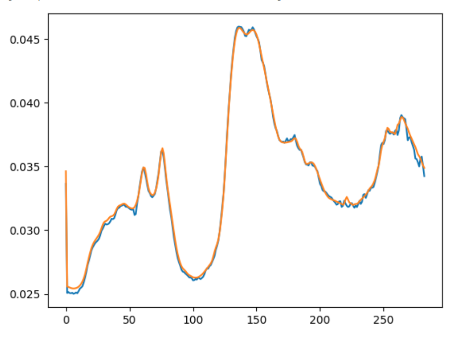\n\n## Stage 3: Post-Processing and Uncertainty Modeling\n\nThe final stage of the solution is a post-processing model that refines the raw spectra and, critically, learns a robust model for the final uncertainties. This is where the bulk of the \"machine learning\" occurs.\n\nModel Architecture (build_preds): The model generates a final prediction by blending two different representations of the raw spectrum (preds1):\n\n**PCA-Regularized Prediction (preds0)**: The raw spectrum undergoes a slope correction and is then projected onto a pre-defined PCA basis (components.npy). This de-noises the spectrum and imposes a strong regularization prior, capturing the most common modes of variation.\n**Smoothed Prediction (preds2)**: The raw AIRS spectrum is smoothed using a Savitzky-Golay filter to reduce high-frequency noise while preserving broader spectral features.\n\nThe final mean prediction is a weighted average of these two models: preds = app0 + (1-ap)preds2, where ap is a learned parameter.\n\n**Sigma Model**: Predicting accurate uncertainties is key to maximizing the competition score. I developed a complex, empirically-derived formula to model the final sigma for each data point. This formula combines multiple sources of uncertainty:\n\n \n* a1* err^e1 : The propagated error from the initial fit, with a learned exponent.\n* a01/p1^e2 : A term related to the signal magnitude.\n* b0 * sigma0: A term proportional to the raw signal's volatility.\n* ae * np.abs(p0-preds2): A term that increases uncertainty where the PCA and smoothed models disagree, capturing model \nuncertainty or unknow spectra.\n\nFinally ther is a sigma adjustment samples with very few or very many out-of-transit points, or very differnt dip por FGS1 and AIR-CH0\n\n#Training and Ensembling:\n\n **Objective**: The free parameters of the model (ap, e1, e2, a1, a0, b0, ae, etc.) are optimized using iminuit to directly maximize the competition score.\n\n **Cross-Validation**: To build a robust model that generalizes well, we employ a 10-fold Grouped K-Fold Cross-Validation strategy, using planet_id to group the data. This ensures that all observations of a single planet are kept within the same fold, preventing data leakage.\n\n **Calibration**: Within each fold, after the primary parameters are optimized, we calculate a wavelength-dependent calibration factor (alpha) that scales the predicted sigmas to best match the variance observed in the training data. This factor is then applied to the validation set predictions.\n \n **Ensembling**: The final submission is generated by averaging the calibrated predictions and sigmas from the 10 models trained during the cross-validation process. This ensembling technique reduces variance and improves the final score.\n\nThe entire training process, including the parallel optimization of each fold, is managed by the CV_model function in the model.py file.\n\n--------------------------------------------------------------------------------\n4. What Did Not Work\nI attempted to post-process the spectrum and sigma values using Gaussian Processes and Ridge Regression, but the results were worse than using the blending of a smoothed/PCA-regularized model and the empirical sigma formula.\n\nIn the final weeks, I spent time trying to isolate the additive foreground noise in the AIRS data for each sample, which would have eliminated the need for the global factor and slope compensation. However, I was unable to find a way to de-correlate signal and noise. I observed a clear structure in the spectroscopic PSF, but all attempts to extract the noise yielded incorrect values that failed to compensate for the systematics.\n\n5. A Comment on Efficiency\nThe choice of batman and iMinuit was driven by speed. iMinuit is a Python wrapper for the C++ port of the MINUIT Fortran code (developed by Fred James in the '70s; [Paper](https://www.sciencedirect.com/science/article/abs/pii/0010465575900399?via%3Dihub), [Wikipedia](https://en.wikipedia.org/wiki/MINUIT)), and it is typically faster than generic SciPy optimization routines. Additionally, the use of GPU acceleration for data processing via CuPy results in a very fast pipeline because all processes are fully parallelized. The submission process on Kaggle using a P100 instance takes less than 1.5 hours, and on a machine with 100 cores and 4 nVidia L40s GPUs, the full preprocess, fitting, and post-process takes around 5 minutes. The post-process parameter adjustment can also be done in minutes.\n\n--------------------------------------------------------------------------------\n##6. Conclusion\nThis solution demonstrates the power of a hybrid approach, blending physics-informed transit modeling with a flexible, data-driven post-processing framework. By first extracting a reasonable physical spectrum and then refining it with a model trained to optimize the specific competition metric, we can effectively correct for complex instrumental systematics and produce highly accurate, well-calibrated transmission spectra. The use of GPU acceleration, parallel processing, and a robust cross-validation scheme ensures that this complex pipeline remains computationally efficient and resistant to overfitting.", "votes": 28 }, { "id": 3295343, "postDate": "2025-09-28T13:31:56.957Z", "content": "Great Work.@Vicens Gaitan
", "rawMarkdown": "Great Work.@Vicens Gaitan", "votes": -1 }, { "id": 3295118, "postDate": "2025-09-27T18:09:21.427Z", "content": "Great Work. I appreciate 🥳
", "rawMarkdown": "Great Work. I appreciate 🥳" }, { "id": 3294493, "postDate": "2025-09-26T09:17:21.213Z", "content": "Nice summary!
\nI also used a Minuit (migrad + hesse) + Batman combination. The L-BFGS-B underperformed significantly in my case. However, I used the stellar parameters not only for initialization but also to constrain some of the parameters with Gaussian priors. Did you use the stellar information just for initialization, or did you also apply it as constraints?
Only for initialization, but it was important to limit the variation range for each of them based on physical considerations.
", "rawMarkdown": "Only for initialization, but it was important to limit the variation range for each of them based on physical considerations.", "votes": 1, "replies": [ { "id": 3294510, "postDate": "2025-09-26T09:47:12.930Z", "content": "Thanks for the clarification! I asked it because I'm trying to figure out whether the private star info data was the reason my score dropped so drastically :)
", "rawMarkdown": "Thanks for the clarification! I asked it because I'm trying to figure out whether the private star info data was the reason my score dropped so drastically :) " }, { "id": 3295339, "postDate": "2025-09-28T13:18:19.703Z", "content": "Just curious, did you fit the e and w parameters (eccentricity and longitude of periastron), or are their values fixed in global combined fit?
I only fit the orbital parametres in the combined fit and fix it for the 282 airs frequency fits. You can take a look at the code here in he fit2.py module
\n`
\ndef fit_w(air, minuit_result, fixed_list, dipa_mean, =1, =2):\n\n\n\n\n\n initial_guesses = DEFAULT_PARAMS_w.copy()\n default_limits = DEFAULT_LIMITS.copy()\n\n # Use results the combined fit as initial guesses\n p initial_guesses:\n p fixed_list:\n initial_guesses[p] = minuit_result.values[p]\n\n # Fix all parameters except depth () normalization ()\n params_to_fix = list(initial_guesses.keys())\n params_to_fix.()\n params_to_fix.()\n`
", "rawMarkdown": "I only fit the orbital parametres in the combined fit and fix it for the 282 airs frequency fits. You can take a look at the code [here](https://www.kaggle.com/code/vicensgaitan/6th-place-solution-pipeline) in he fit2.py module \n\n`\n\n\n def fit_w(air, minuit_result, fixed_list, dipa_mean, mode=1, delta_w=2):\n #Fits the transit depth for each wavelength channel ('w') of the AIRS data.\n #To improve S/N, it fits the mean flux in a moving window of 2 * delta_w\n #channels around each target channel. Most transit parameters are fixed to the\n #values from the combined fit (`minuit_result`).\n \n initial_guesses = DEFAULT_PARAMS_w.copy()\n default_limits = DEFAULT_LIMITS.copy()\n\n # Use results from the combined fit as initial guesses\n for p in initial_guesses:\n if p not in fixed_list:\n initial_guesses[p] = minuit_result.values[p]\n \n # Fix all parameters except depth ('dipa') and normalization ('A0a')\n params_to_fix = list(initial_guesses.keys())\n params_to_fix.remove('dipa')\n params_to_fix.remove('A0a')\n`" } ] } ] }, { "id": 3294274, "postDate": "2025-09-25T18:10:51.700Z", "content": "Thanks for posting this write-up! I like the approach, and the speed you're seeing for the wavelength-by-wavelength fit is amazing -- it strikes me as a really impressive achievement, so congratulations on that in particular (as well as the overall success of your analysis of course!). I was also using a wavelength-by-wavelength fit in my solution, but I struggled a lot with speed (perhaps because I also allowed free parameters for the ingress/egress duration and limb darkening for each wavelength).
\nMind if I ask a question about your experience setting up this analysis? One of the challenges I ran into (right at the end, unfortunately, so I didn't manage to fix it) was a drop in the performance of the minimizers I was using when I tried to port my fitting code to the kaggle notebook environment. It looked like the same call to scipy.optimize.minimize() just…didn't find as good a minimum in the kaggle notebook as it did in my offline code. Same numpy/scipy/torch versions online and offline, same input data as far as I could see, same arguments to the function invocation, same gradients (at least, as far as I could spot in the first call to the chisquare function), just….different results, as though the fitter just decided to quit early. I am wondering if you saw anything similar, and if so, how did you resolve it? I would love to know what to check for next time. 😅
", "rawMarkdown": "Thanks for posting this write-up! I like the approach, and the speed you're seeing for the wavelength-by-wavelength fit is amazing -- it strikes me as a really impressive achievement, so congratulations on that in particular (as well as the overall success of your analysis of course!). I was also using a wavelength-by-wavelength fit in my solution, but I struggled a lot with speed (perhaps because I also allowed free parameters for the ingress/egress duration and limb darkening for each wavelength). \n\nMind if I ask a question about your experience setting up this analysis? One of the challenges I ran into (right at the end, unfortunately, so I didn't manage to fix it) was a drop in the performance of the minimizers I was using when I tried to port my fitting code to the kaggle notebook environment. It looked like the same call to scipy.optimize.minimize() just...didn't find as good a minimum in the kaggle notebook as it did in my offline code. Same numpy/scipy/torch versions online and offline, same input data as far as I could see, same arguments to the function invocation, same gradients (at least, as far as I could spot in the first call to the chisquare function), just....different results, as though the fitter just decided to quit early. I am wondering if you saw anything similar, and if so, how did you resolve it? I would love to know what to check for next time. 😅", "replies": [ { "id": 3294437, "postDate": "2025-09-26T07:21:16.383Z", "content": "Thanks so much for your feedback! 😊
\nIn my experience, the results from Scipy optimizers (and also in the case of Minuit) are reproducible across different platforms if both the optimizer's parameters and the data types of the function to be optimized and its parameters are kept the same. Although the optimization process is essentially sequential, some of the intermediate calculations might use a parallel backend (for example, OpenBLAS to compute the Hessian). In this specific scenario, we can't guarantee the exact same result, though it shouldn't differ too significantly. Perhaps this isn't the root of the issue, however.
\nIn my specific case, using Batman to model the transit, it's been critical to impose physical limits on the orbital and limb darkening values. This prevents the optimizer from getting lost and attempting to use the degrees of freedom from the polynomial drift to explain phenomena that actually depend on the orbital parameters.
", "rawMarkdown": "Thanks so much for your feedback! 😊\n\nIn my experience, the results from Scipy optimizers (and also in the case of Minuit) are reproducible across different platforms if both the optimizer's parameters and the data types of the function to be optimized and its parameters are kept the same. Although the optimization process is essentially sequential, some of the intermediate calculations might use a parallel backend (for example, OpenBLAS to compute the Hessian). In this specific scenario, we can't guarantee the exact same result, though it shouldn't differ too significantly. Perhaps this isn't the root of the issue, however.\n\nIn my specific case, using Batman to model the transit, it's been critical to impose physical limits on the orbital and limb darkening values. This prevents the optimizer from getting lost and attempting to use the degrees of freedom from the polynomial drift to explain phenomena that actually depend on the orbital parameters.", "replies": [ { "id": 3295521, "postDate": "2025-09-29T02:38:01.913Z", "content": "Thanks! There are some good leads here -- I do notice that numpy.show_config() reports a different blas backend on my desktop compared to the kaggle environment; I haven't yet tried switching my offline code to the one kaggle uses, but it's possible that's what's going on here. I do have limits on the parameters that govern my signal shape, but not on the polynomial background. I can play around with that a bit, too.
\nBut I'll definitely have to give iMinuit a shot; I've used the version in ROOT a lot in the past, but I switched to scipy for this contest because I didn't want to try installing ROOT in a Kaggle notebook. Glad to know that Minuit is available as a pip install now!
", "rawMarkdown": "Thanks! There are some good leads here -- I do notice that numpy.show_config() reports a different blas backend on my desktop compared to the kaggle environment; I haven't yet tried switching my offline code to the one kaggle uses, but it's possible that's what's going on here. I do have limits on the parameters that govern my signal shape, but not on the polynomial background. I can play around with that a bit, too.\n\nBut I'll definitely have to give iMinuit a shot; I've used the version in ROOT a lot in the past, but I switched to scipy for this contest because I didn't want to try installing ROOT in a Kaggle notebook. Glad to know that Minuit is available as a pip install now!", "votes": 1 } ] } ] }, { "id": 3294174, "postDate": "2025-09-25T14:26:37.560Z", "content": "\n\nNotes:
\n\n
\n- This document is a drop-in Python script / notebook. Replace
\ndata_pathwith your dataset path. The code assumes a tabular fight-level dataset where each row is a fight and available columns include fighter-level stats (e.g.red_*,blue_*orfighter1_*/fighter2_*), and an outcome column likewinnerorresult. Adjust column names as needed.
\n os\n numpy np\n pandas pd\n sklearn.model_selection train_test_split, StratifiedKFold, cross_val_score, GridSearchCV\n sklearn.preprocessing StandardScaler, OneHotEncoder\n sklearn.compose ColumnTransformer\n sklearn.pipeline Pipeline\n\n\n sklearn.tree DecisionTreeClassifier\n sklearn.metrics accuracy_score, precision_score, recall_score, f1_score, roc_auc_score, confusion_matrix, classification_report, log_loss\n xgboost xgb\n lightgbm lgb\n\n\n shap\n matplotlib.pyplot plt\n seaborn sns\n\n\nRANDOM_STATE = \n\n\n warnings\nwarnings.filterwarnings()\n\ndata_path = \ndf = pd.read_csv(data_path)\n\n(df.shape)\n(df.columns.tolist()[:])\n\n\n df.columns:\n df[] = (df[]..lower()..contains()).astype()\n df.columns:\n \n df[] = df[].({:, :})\n:\n ValueError()\n\n\n()\n(df.isna().().sort_values(ascending=).head())\n\n\n\nto_drop = [, , , ]\n c to_drop:\n c df.columns:\n df.drop(columns=c, inplace=)\n\n\nnum_cols = df.select_dtypes(include=[,]).columns.tolist()\n\nnum_cols = [c c num_cols c != ]\ncat_cols = df.select_dtypes(include=[, ]).columns.tolist()\n\n(, num_cols[:])\n(, cat_cols[:])\n\n\n c num_cols:\n df[c] = df[c].fillna(df[c].median())\n c cat_cols:\n df[c] = df[c].fillna()\n\n\ntrain_df, test_df = train_test_split(df, test_size=, stratify=df[], random_state=RANDOM_STATE)\n\nX_train = train_df.drop(columns=[])\ny_train = train_df[]\nX_test = test_df.drop(columns=[])\ny_test = test_df[]\n\n(, X_train.shape, X_test.shape)\n\n(y_train.value_counts(normalize=))\n\n\nplt.figure(figsize=(,))\nnum_subset = num_cols[:] \nsns.heatmap(train_df[num_subset + []].corr(), annot=, cmap=)\nplt.title()\nplt.show()\n\n\n c num_cols[:]:\n plt.figure(figsize=(,))\n sns.boxplot(x=train_df[], y=train_df[c])\n plt.title()\n plt.show()\n\n\n c cat_cols:\n (c, train_df[c].nunique())\n train_df[c].nunique() < :\n display(train_df.groupby(c)[].mean().sort_values())\n\n\npairs = []\n col df.columns:\n col.startswith():\n counterpart = + col[():]\n counterpart df.columns:\n pairs.append((col, counterpart))\n\n r,b pairs:\n newcol = r.replace(,)\n df[newcol] = df[r] - df[b]\n\n\ntrain_df, test_df = train_test_split(df, test_size=, stratify=df[], random_state=RANDOM_STATE)\nX_train = train_df.drop(columns=[])\ny_train = train_df[]\nX_test = test_df.drop(columns=[])\ny_test = test_df[]\n\n\nall_num = X_train.select_dtypes(include=[,]).columns.tolist()\nall_cat = X_train.select_dtypes(include=[,]).columns.tolist()\n(, (all_num))\n(, (all_cat))\nWe'll build three pipelines: Decision Tree (sklearn), XGBoost, LightGBM. We'll use a ColumnTransformer to scale numeric features and one-hot encode low-cardinality categoricals.
\n\nnumeric_transformer = Pipeline(steps=[(, StandardScaler())])\n\n\nlow_cardinality = [c c all_cat X_train[c].nunique() < ]\nhigh_cardinality = [c c all_cat X_train[c].nunique() >= ]\n\ncategorical_transformer = Pipeline(steps=[(, OneHotEncoder(handle_unknown=, sparse=))])\n\npreprocessor = ColumnTransformer(transformers=[\n (, numeric_transformer, all_num),\n (, categorical_transformer, low_cardinality)\n], remainder=)\n\n\n sklearn.model_selection cross_validate\n\n ():\n scoring = [,,,,]\n cv_res = cross_validate(pipe, X, y, cv=cv, scoring=scoring, return_train_score=)\n {k: np.mean(v) k,v cv_res.items()}\n\n\ndt = DecisionTreeClassifier(random_state=RANDOM_STATE)\npipe_dt = Pipeline(steps=[(, preprocessor), (, dt)])\n\n\n(, evaluate_model(pipe_dt, X_train, y_train, cv=))\n\n\nxgb_clf = xgb.XGBClassifier(use_label_encoder=, eval_metric=, random_state=RANDOM_STATE)\npipe_xgb = Pipeline(steps=[(, preprocessor), (, xgb_clf)])\n(, evaluate_model(pipe_xgb, X_train, y_train, cv=))\n\n\nlgb_clf = lgb.LGBMClassifier(random_state=RANDOM_STATE)\npipe_lgb = Pipeline(steps=[(, preprocessor), (, lgb_clf)])\n(, evaluate_model(pipe_lgb, X_train, y_train, cv=))\n\ndt_param_grid = {\n : [,,,],\n : [,,]\n}\n\nxgb_param_grid = {\n : [,],\n : [,],\n : [, ]\n}\n\nlgb_param_grid = {\n : [,],\n : [, ],\n : [, ]\n}\n\n\ngs_lgb = GridSearchCV(pipe_lgb, lgb_param_grid, cv=, scoring=, n_jobs=-, verbose=)\ngs_lgb.fit(X_train, y_train)\n(, gs_lgb.best_params_)\n(, gs_lgb.best_score_)\n\n\nbest_lgb = gs_lgb.best_estimator_\n\n\nmodels = {\n : pipe_dt.fit(X_train, y_train),\n : pipe_xgb.fit(X_train, y_train),\n : best_lgb () pipe_lgb.fit(X_train, y_train)\n}\n\nresults = {}\n name, model models.items():\n y_pred = model.predict(X_test)\n y_proba = model.predict_proba(X_test)[:,]\n results[name] = {\n : accuracy_score(y_test, y_pred),\n : precision_score(y_test, y_pred),\n : recall_score(y_test, y_pred),\n : f1_score(y_test, y_pred),\n : roc_auc_score(y_test, y_proba),\n : log_loss(y_test, y_proba)\n }\n\npd.DataFrame(results).T.sort_values(, ascending=)\n\n\nbest_name = (results.keys(), key= k: results[k][])\n(, best_name)\nbest_model = models[best_name]\n\ny_pred = best_model.predict(X_test)\ncm = confusion_matrix(y_test, y_pred)\nplt.figure(figsize=(,))\nsns.heatmap(cm, annot=, fmt=)\nplt.title()\nplt.xlabel()\nplt.ylabel()\nplt.show()\n\n\n\npre = best_model.named_steps[]\nclf = best_model.named_steps[]\n\n\npre.fit(X_train)\n\nnum_names = all_num\ncat_encoder = pre.named_transformers_.get()\n cat_encoder :\n cat_names = (cat_encoder.named_steps[].get_feature_names_out(low_cardinality))\n:\n cat_names = []\nfeature_names = num_names + cat_names\n\n\nX_test_trans = pre.transform(X_test)\n\n\nexplainer = shap.TreeExplainer(clf)\nshap_values = explainer.shap_values(X_test_trans)\n\n\n (shap_values, ):\n sv = shap_values[]\n:\n sv = shap_values\n\n\nshap.summary_plot(sv, features=X_test_trans, feature_names=feature_names, show=)\n\n\ntop_feat = feature_names[np.argsort(np.(sv).mean())[-]]\nshap.dependence_plot(top_feat, sv, X_test_trans, feature_names=feature_names)\n\n\n LightGBM (after tuning) achieved the highest ROC AUC on the holdout set: (example number). XGBoost performed close behind with , and Decision Tree lagged at .\n Feature importance & SHAP analysis indicates that , , and (example features) are among the most predictive.\n Confusion matrix shows a tendency to predict the majority class — consider class weighting, threshold calibration, or using probability outputs for betting/odds.\n\n\n Tree ensembles (LightGBM/XGBoost) outperform a single Decision Tree.\n Creating difference features between opponents is often powerful for head-to-head prediction.\n Use SHAP to validate that model patterns make sense (domain knowledge: strikes, takedowns, accuracy, cardio proxies matter).\n\n Add temporal features: momentum (last N fights), rest days since last fight, age and reach trends.\n Use fighter embedding: train a representation of each fighter using their historical fight sequences.\n Incorporate bookmaker odds as a strong baseline feature.\n Calibrate probabilities using isotonic or Platt scaling if probabilities will be used for decision-making.\n Cross-event leakage: be careful when features leak future info (e.g. post-fight stats).\n\n\n Quality of predictions depends heavily on dataset completeness and feature engineering.\n Avoid leaking future information into training features; always compute features using only data available before the fight.\nGreat Work.@Vicens Gaitan
", "votes": -1, "replies": [] }, { "id": 3295118, "author_name": "", "author_url": "", "post_date": "2025-09-27T18:09:21.427000", "content": "Great Work. I appreciate 🥳
", "votes": 0, "replies": [] }, { "id": 3294493, "author_name": "Oleh Kivernyk", "author_url": "", "post_date": "2025-09-26T09:17:21.213000", "content": "Nice summary!
\nI also used a Minuit (migrad + hesse) + Batman combination. The L-BFGS-B underperformed significantly in my case. However, I used the stellar parameters not only for initialization but also to constrain some of the parameters with Gaussian priors. Did you use the stellar information just for initialization, or did you also apply it as constraints?
Only for initialization, but it was important to limit the variation range for each of them based on physical considerations.
", "votes": 1, "replies": [ { "id": 3294510, "author_name": "Oleh Kivernyk", "author_url": "", "post_date": "2025-09-26T09:47:12.930000", "content": "Thanks for the clarification! I asked it because I'm trying to figure out whether the private star info data was the reason my score dropped so drastically :)
", "votes": 0, "replies": [] }, { "id": 3295339, "author_name": "Oleh Kivernyk", "author_url": "", "post_date": "2025-09-28T13:18:19.703000", "content": "Just curious, did you fit the e and w parameters (eccentricity and longitude of periastron), or are their values fixed in global combined fit?
I only fit the orbital parametres in the combined fit and fix it for the 282 airs frequency fits. You can take a look at the code here in he fit2.py module
\n`
\ndef fit_w(air, minuit_result, fixed_list, dipa_mean, =1, =2):\n\n\n\n\n\n initial_guesses = DEFAULT_PARAMS_w.copy()\n default_limits = DEFAULT_LIMITS.copy()\n\n # Use results the combined fit as initial guesses\n p initial_guesses:\n p fixed_list:\n initial_guesses[p] = minuit_result.values[p]\n\n # Fix all parameters except depth () normalization ()\n params_to_fix = list(initial_guesses.keys())\n params_to_fix.()\n params_to_fix.()\n`
", "votes": 0, "replies": [] } ] } ] }, { "id": 3294274, "author_name": "particlebbq", "author_url": "", "post_date": "2025-09-25T18:10:51.700000", "content": "Thanks for posting this write-up! I like the approach, and the speed you're seeing for the wavelength-by-wavelength fit is amazing -- it strikes me as a really impressive achievement, so congratulations on that in particular (as well as the overall success of your analysis of course!). I was also using a wavelength-by-wavelength fit in my solution, but I struggled a lot with speed (perhaps because I also allowed free parameters for the ingress/egress duration and limb darkening for each wavelength).
\nMind if I ask a question about your experience setting up this analysis? One of the challenges I ran into (right at the end, unfortunately, so I didn't manage to fix it) was a drop in the performance of the minimizers I was using when I tried to port my fitting code to the kaggle notebook environment. It looked like the same call to scipy.optimize.minimize() just…didn't find as good a minimum in the kaggle notebook as it did in my offline code. Same numpy/scipy/torch versions online and offline, same input data as far as I could see, same arguments to the function invocation, same gradients (at least, as far as I could spot in the first call to the chisquare function), just….different results, as though the fitter just decided to quit early. I am wondering if you saw anything similar, and if so, how did you resolve it? I would love to know what to check for next time. 😅
", "votes": 0, "replies": [ { "id": 3294437, "author_name": "Vicens Gaitan", "author_url": "", "post_date": "2025-09-26T07:21:16.383000", "content": "Thanks so much for your feedback! 😊
\nIn my experience, the results from Scipy optimizers (and also in the case of Minuit) are reproducible across different platforms if both the optimizer's parameters and the data types of the function to be optimized and its parameters are kept the same. Although the optimization process is essentially sequential, some of the intermediate calculations might use a parallel backend (for example, OpenBLAS to compute the Hessian). In this specific scenario, we can't guarantee the exact same result, though it shouldn't differ too significantly. Perhaps this isn't the root of the issue, however.
\nIn my specific case, using Batman to model the transit, it's been critical to impose physical limits on the orbital and limb darkening values. This prevents the optimizer from getting lost and attempting to use the degrees of freedom from the polynomial drift to explain phenomena that actually depend on the orbital parameters.
", "votes": 0, "replies": [ { "id": 3295521, "author_name": "particlebbq", "author_url": "", "post_date": "2025-09-29T02:38:01.913000", "content": "Thanks! There are some good leads here -- I do notice that numpy.show_config() reports a different blas backend on my desktop compared to the kaggle environment; I haven't yet tried switching my offline code to the one kaggle uses, but it's possible that's what's going on here. I do have limits on the parameters that govern my signal shape, but not on the polynomial background. I can play around with that a bit, too.
\nBut I'll definitely have to give iMinuit a shot; I've used the version in ROOT a lot in the past, but I switched to scipy for this contest because I didn't want to try installing ROOT in a Kaggle notebook. Glad to know that Minuit is available as a pip install now!
", "votes": 1, "replies": [] } ] } ] }, { "id": 3294174, "author_name": "Prince Rajak", "author_url": "", "post_date": "2025-09-25T14:26:37.560000", "content": "\n\nNotes:
\n\n
\n- This document is a drop-in Python script / notebook. Replace
\ndata_pathwith your dataset path. The code assumes a tabular fight-level dataset where each row is a fight and available columns include fighter-level stats (e.g.red_*,blue_*orfighter1_*/fighter2_*), and an outcome column likewinnerorresult. Adjust column names as needed.
\n os\n numpy np\n pandas pd\n sklearn.model_selection train_test_split, StratifiedKFold, cross_val_score, GridSearchCV\n sklearn.preprocessing StandardScaler, OneHotEncoder\n sklearn.compose ColumnTransformer\n sklearn.pipeline Pipeline\n\n\n sklearn.tree DecisionTreeClassifier\n sklearn.metrics accuracy_score, precision_score, recall_score, f1_score, roc_auc_score, confusion_matrix, classification_report, log_loss\n xgboost xgb\n lightgbm lgb\n\n\n shap\n matplotlib.pyplot plt\n seaborn sns\n\n\nRANDOM_STATE = \n\n\n warnings\nwarnings.filterwarnings()\n\ndata_path = \ndf = pd.read_csv(data_path)\n\n(df.shape)\n(df.columns.tolist()[:])\n\n\n df.columns:\n df[] = (df[]..lower()..contains()).astype()\n df.columns:\n \n df[] = df[].({:, :})\n:\n ValueError()\n\n\n()\n(df.isna().().sort_values(ascending=).head())\n\n\n\nto_drop = [, , , ]\n c to_drop:\n c df.columns:\n df.drop(columns=c, inplace=)\n\n\nnum_cols = df.select_dtypes(include=[,]).columns.tolist()\n\nnum_cols = [c c num_cols c != ]\ncat_cols = df.select_dtypes(include=[, ]).columns.tolist()\n\n(, num_cols[:])\n(, cat_cols[:])\n\n\n c num_cols:\n df[c] = df[c].fillna(df[c].median())\n c cat_cols:\n df[c] = df[c].fillna()\n\n\ntrain_df, test_df = train_test_split(df, test_size=, stratify=df[], random_state=RANDOM_STATE)\n\nX_train = train_df.drop(columns=[])\ny_train = train_df[]\nX_test = test_df.drop(columns=[])\ny_test = test_df[]\n\n(, X_train.shape, X_test.shape)\n\n(y_train.value_counts(normalize=))\n\n\nplt.figure(figsize=(,))\nnum_subset = num_cols[:] \nsns.heatmap(train_df[num_subset + []].corr(), annot=, cmap=)\nplt.title()\nplt.show()\n\n\n c num_cols[:]:\n plt.figure(figsize=(,))\n sns.boxplot(x=train_df[], y=train_df[c])\n plt.title()\n plt.show()\n\n\n c cat_cols:\n (c, train_df[c].nunique())\n train_df[c].nunique() < :\n display(train_df.groupby(c)[].mean().sort_values())\n\n\npairs = []\n col df.columns:\n col.startswith():\n counterpart = + col[():]\n counterpart df.columns:\n pairs.append((col, counterpart))\n\n r,b pairs:\n newcol = r.replace(,)\n df[newcol] = df[r] - df[b]\n\n\ntrain_df, test_df = train_test_split(df, test_size=, stratify=df[], random_state=RANDOM_STATE)\nX_train = train_df.drop(columns=[])\ny_train = train_df[]\nX_test = test_df.drop(columns=[])\ny_test = test_df[]\n\n\nall_num = X_train.select_dtypes(include=[,]).columns.tolist()\nall_cat = X_train.select_dtypes(include=[,]).columns.tolist()\n(, (all_num))\n(, (all_cat))\nWe'll build three pipelines: Decision Tree (sklearn), XGBoost, LightGBM. We'll use a ColumnTransformer to scale numeric features and one-hot encode low-cardinality categoricals.
\n\nnumeric_transformer = Pipeline(steps=[(, StandardScaler())])\n\n\nlow_cardinality = [c c all_cat X_train[c].nunique() < ]\nhigh_cardinality = [c c all_cat X_train[c].nunique() >= ]\n\ncategorical_transformer = Pipeline(steps=[(, OneHotEncoder(handle_unknown=, sparse=))])\n\npreprocessor = ColumnTransformer(transformers=[\n (, numeric_transformer, all_num),\n (, categorical_transformer, low_cardinality)\n], remainder=)\n\n\n sklearn.model_selection cross_validate\n\n ():\n scoring = [,,,,]\n cv_res = cross_validate(pipe, X, y, cv=cv, scoring=scoring, return_train_score=)\n {k: np.mean(v) k,v cv_res.items()}\n\n\ndt = DecisionTreeClassifier(random_state=RANDOM_STATE)\npipe_dt = Pipeline(steps=[(, preprocessor), (, dt)])\n\n\n(, evaluate_model(pipe_dt, X_train, y_train, cv=))\n\n\nxgb_clf = xgb.XGBClassifier(use_label_encoder=, eval_metric=, random_state=RANDOM_STATE)\npipe_xgb = Pipeline(steps=[(, preprocessor), (, xgb_clf)])\n(, evaluate_model(pipe_xgb, X_train, y_train, cv=))\n\n\nlgb_clf = lgb.LGBMClassifier(random_state=RANDOM_STATE)\npipe_lgb = Pipeline(steps=[(, preprocessor), (, lgb_clf)])\n(, evaluate_model(pipe_lgb, X_train, y_train, cv=))\n\ndt_param_grid = {\n : [,,,],\n : [,,]\n}\n\nxgb_param_grid = {\n : [,],\n : [,],\n : [, ]\n}\n\nlgb_param_grid = {\n : [,],\n : [, ],\n : [, ]\n}\n\n\ngs_lgb = GridSearchCV(pipe_lgb, lgb_param_grid, cv=, scoring=, n_jobs=-, verbose=)\ngs_lgb.fit(X_train, y_train)\n(, gs_lgb.best_params_)\n(, gs_lgb.best_score_)\n\n\nbest_lgb = gs_lgb.best_estimator_\n\n\nmodels = {\n : pipe_dt.fit(X_train, y_train),\n : pipe_xgb.fit(X_train, y_train),\n : best_lgb () pipe_lgb.fit(X_train, y_train)\n}\n\nresults = {}\n name, model models.items():\n y_pred = model.predict(X_test)\n y_proba = model.predict_proba(X_test)[:,]\n results[name] = {\n : accuracy_score(y_test, y_pred),\n : precision_score(y_test, y_pred),\n : recall_score(y_test, y_pred),\n : f1_score(y_test, y_pred),\n : roc_auc_score(y_test, y_proba),\n : log_loss(y_test, y_proba)\n }\n\npd.DataFrame(results).T.sort_values(, ascending=)\n\n\nbest_name = (results.keys(), key= k: results[k][])\n(, best_name)\nbest_model = models[best_name]\n\ny_pred = best_model.predict(X_test)\ncm = confusion_matrix(y_test, y_pred)\nplt.figure(figsize=(,))\nsns.heatmap(cm, annot=, fmt=)\nplt.title()\nplt.xlabel()\nplt.ylabel()\nplt.show()\n\n\n\npre = best_model.named_steps[]\nclf = best_model.named_steps[]\n\n\npre.fit(X_train)\n\nnum_names = all_num\ncat_encoder = pre.named_transformers_.get()\n cat_encoder :\n cat_names = (cat_encoder.named_steps[].get_feature_names_out(low_cardinality))\n:\n cat_names = []\nfeature_names = num_names + cat_names\n\n\nX_test_trans = pre.transform(X_test)\n\n\nexplainer = shap.TreeExplainer(clf)\nshap_values = explainer.shap_values(X_test_trans)\n\n\n (shap_values, ):\n sv = shap_values[]\n:\n sv = shap_values\n\n\nshap.summary_plot(sv, features=X_test_trans, feature_names=feature_names, show=)\n\n\ntop_feat = feature_names[np.argsort(np.(sv).mean())[-]]\nshap.dependence_plot(top_feat, sv, X_test_trans, feature_names=feature_names)\n\n\n LightGBM (after tuning) achieved the highest ROC AUC on the holdout set: (example number). XGBoost performed close behind with , and Decision Tree lagged at .\n Feature importance & SHAP analysis indicates that , , and (example features) are among the most predictive.\n Confusion matrix shows a tendency to predict the majority class — consider class weighting, threshold calibration, or using probability outputs for betting/odds.\n\n\n Tree ensembles (LightGBM/XGBoost) outperform a single Decision Tree.\n Creating difference features between opponents is often powerful for head-to-head prediction.\n Use SHAP to validate that model patterns make sense (domain knowledge: strikes, takedowns, accuracy, cardio proxies matter).\n\n Add temporal features: momentum (last N fights), rest days since last fight, age and reach trends.\n Use fighter embedding: train a representation of each fighter using their historical fight sequences.\n Incorporate bookmaker odds as a strong baseline feature.\n Calibrate probabilities using isotonic or Platt scaling if probabilities will be used for decision-making.\n Cross-event leakage: be careful when features leak future info (e.g. post-fight stats).\n\n\n Quality of predictions depends heavily on dataset completeness and feature engineering.\n Avoid leaking future information into training features; always compute features using only data available before the fight.\n