
First, I would like to thank the organizers for this great competition!
\nMy solution uses linear regression with transit depth estimation based on polynomial fitting. I didn't model the full physics of transits, but created features that capture transit shape patterns from light curves.
\nI used the standard preprocessing provided by the competition without additional steps.
\nMost features are based on polynomial fitting. I found transit boundaries by detecting 4 extrema of the second derivative - points where the light curve curvature changes most rapidly. For depth estimation and detrending, I fit a polynomial of chosen degree to out-of-transit points and divide the curve by this interpolation.
\n
The features fall into three main groups. First: depth estimates from AIRS frequencies averaged with SNR weights, inspired by last year's solutions. Second: depth estimates from intersecting windows across adjacent AIRS frequencies. Third: depth estimates from the FG1 channel separately.
\nFor the SNR-weighted group, I optimized polynomial degree (1-5) minimizing: err = RMSE × degree^(n_transit / n_total) where RMSE is calculated between the original curve and polynomial interpolation in out-of-transit regions, degree is the polynomial degree used for fitting, n_transit is the number of points inside the transit, and n_total is the total number of observation points. When transits occupy more of the observation, fewer points are available for baseline fitting, making higher degrees less reliable. This optimization gave only small improvement on private leaderboard. For other groups, I used fixed degree 3.
\nFor each of these three feature groups (AIRS averaged, AIRS windowed, FG1), I calculated multiple depth values: average across transit, mid-transit, and various percentiles. For frequency windows with too much noise, I didn't use polynomial interpolation but instead used a rough estimate based on the ratio of average flux inside and outside the transit.
\nI also computed slope features for the SNR-weighted AIRS and FG1 groups only - these measure wall steepness as flux change rate between boundary points. Another small group used remaining physical information but provided little improvement.
\n%20%20.png?generation=1759414981223394&alt=media\")
I identified transits near observation edges as outliers and trained a separate Ridge model for them. The outlier model was trained on all data, while the main model used only normal cases. For very poor quality transits, I removed them during training and used larger sigma values for inference.
\nFor uncertainty estimation, I used bootstrapping: created multiple resampled datasets, trained models on each, took standard deviation of all model predictions, and multiplied by an optimized constant. This was combined linearly with cross-validation standard deviations averaged per frequency.
\nDue to metric instability, results might improve with small feature and hyperparameter tuning.
\n| Method | \nPublic Score | \nPrivate Score | \n
|---|---|---|
| Full solution | \n60.9 | \n61.2 | \n
| No SNR-weighted averaging | \n60.6 | \n61.0 | \n
| No slope features | \n52.6 | \n54.1 | \n
| No bootstrapping | \n46.3 | \n57.6 | \n
| No degree optimizing | \n60.4 | \n61.1 | \n
| No physical features | \n60.2 | \n61.2 | \n
| No percentile features | \n57.5 | \n57.2 | \n
In \"no bootstrapping\", I used RMSE estimates from validation, multiplied by 5 for outliers to prevent zero scores. In \"no percentile features\", I kept only average and mid-transit depth measurements.
\nAdditional implementation details can be found in the notebook.
", "messages": [ { "id": 3297294, "postDate": "2025-10-02T19:39:03.053Z", "content": "\nFirst, I would like to thank the organizers for this great competition!
\nMy solution uses linear regression with transit depth estimation based on polynomial fitting. I didn't model the full physics of transits, but created features that capture transit shape patterns from light curves.
\nI used the standard preprocessing provided by the competition without additional steps.
\nMost features are based on polynomial fitting. I found transit boundaries by detecting 4 extrema of the second derivative - points where the light curve curvature changes most rapidly. For depth estimation and detrending, I fit a polynomial of chosen degree to out-of-transit points and divide the curve by this interpolation.
\n
The features fall into three main groups. First: depth estimates from AIRS frequencies averaged with SNR weights, inspired by last year's solutions. Second: depth estimates from intersecting windows across adjacent AIRS frequencies. Third: depth estimates from the FG1 channel separately.
\nFor the SNR-weighted group, I optimized polynomial degree (1-5) minimizing: err = RMSE × degree^(n_transit / n_total) where RMSE is calculated between the original curve and polynomial interpolation in out-of-transit regions, degree is the polynomial degree used for fitting, n_transit is the number of points inside the transit, and n_total is the total number of observation points. When transits occupy more of the observation, fewer points are available for baseline fitting, making higher degrees less reliable. This optimization gave only small improvement on private leaderboard. For other groups, I used fixed degree 3.
\nFor each of these three feature groups (AIRS averaged, AIRS windowed, FG1), I calculated multiple depth values: average across transit, mid-transit, and various percentiles. For frequency windows with too much noise, I didn't use polynomial interpolation but instead used a rough estimate based on the ratio of average flux inside and outside the transit.
\nI also computed slope features for the SNR-weighted AIRS and FG1 groups only - these measure wall steepness as flux change rate between boundary points. Another small group used remaining physical information but provided little improvement.
\n
I identified transits near observation edges as outliers and trained a separate Ridge model for them. The outlier model was trained on all data, while the main model used only normal cases. For very poor quality transits, I removed them during training and used larger sigma values for inference.
\nFor uncertainty estimation, I used bootstrapping: created multiple resampled datasets, trained models on each, took standard deviation of all model predictions, and multiplied by an optimized constant. This was combined linearly with cross-validation standard deviations averaged per frequency.
\nDue to metric instability, results might improve with small feature and hyperparameter tuning.
\n| Method | \nPublic Score | \nPrivate Score | \n
|---|---|---|
| Full solution | \n60.9 | \n61.2 | \n
| No SNR-weighted averaging | \n60.6 | \n61.0 | \n
| No slope features | \n52.6 | \n54.1 | \n
| No bootstrapping | \n46.3 | \n57.6 | \n
| No degree optimizing | \n60.4 | \n61.1 | \n
| No physical features | \n60.2 | \n61.2 | \n
| No percentile features | \n57.5 | \n57.2 | \n
In \"no bootstrapping\", I used RMSE estimates from validation, multiplied by 5 for outliers to prevent zero scores. In \"no percentile features\", I kept only average and mid-transit depth measurements.
\nAdditional implementation details can be found in the notebook.
", "rawMarkdown": "[Submission notebook link](https://www.kaggle.com/code/beemax/neurips-adc-25-2nd-place-submission)\n\n## Introduction\n\nFirst, I would like to thank the organizers for this great competition!\n\nMy solution uses linear regression with transit depth estimation based on polynomial fitting. I didn't model the full physics of transits, but created features that capture transit shape patterns from light curves.\n\n## Data Preprocessing\n\nI used the standard preprocessing provided by the competition without additional steps.\n\n## Feature Engineering\n\nMost features are based on polynomial fitting. I found transit boundaries by detecting 4 extrema of the second derivative - points where the light curve curvature changes most rapidly. For depth estimation and detrending, I fit a polynomial of chosen degree to out-of-transit points and divide the curve by this interpolation.\n\n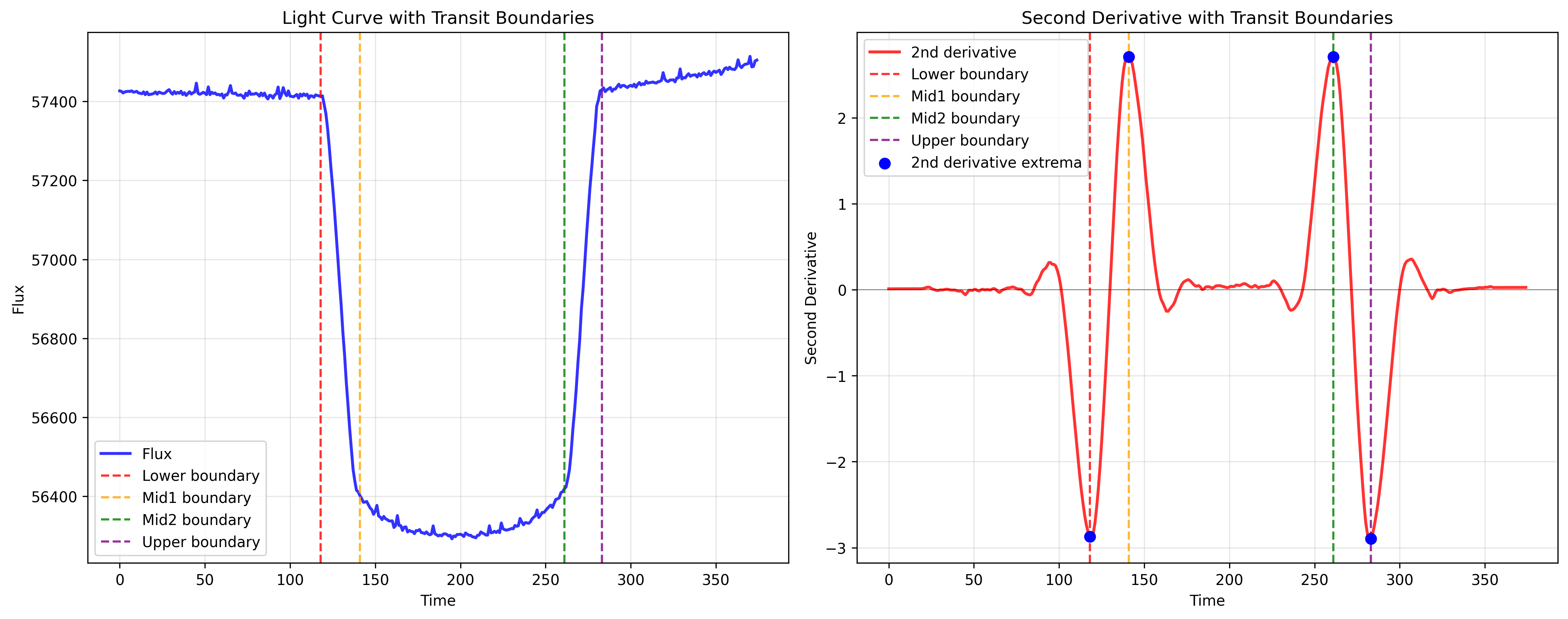\n\nThe features fall into three main groups. First: depth estimates from AIRS frequencies averaged with SNR weights, inspired by last year's solutions. Second: depth estimates from intersecting windows across adjacent AIRS frequencies. Third: depth estimates from the FG1 channel separately.\n\nFor the SNR-weighted group, I optimized polynomial degree (1-5) minimizing: err = RMSE × degree^(n_transit / n_total) where RMSE is calculated between the original curve and polynomial interpolation in out-of-transit regions, degree is the polynomial degree used for fitting, n_transit is the number of points inside the transit, and n_total is the total number of observation points. When transits occupy more of the observation, fewer points are available for baseline fitting, making higher degrees less reliable. This optimization gave only small improvement on private leaderboard. For other groups, I used fixed degree 3.\n\nFor each of these three feature groups (AIRS averaged, AIRS windowed, FG1), I calculated multiple depth values: average across transit, mid-transit, and various percentiles. For frequency windows with too much noise, I didn't use polynomial interpolation but instead used a rough estimate based on the ratio of average flux inside and outside the transit.\n\nI also computed slope features for the SNR-weighted AIRS and FG1 groups only - these measure wall steepness as flux change rate between boundary points. Another small group used remaining physical information but provided little improvement.\n\n%20%20.png?generation=1759414981223394&alt=media)\n\n## Outlier Processing\n\nI identified transits near observation edges as outliers and trained a separate Ridge model for them. The outlier model was trained on all data, while the main model used only normal cases. For very poor quality transits, I removed them during training and used larger sigma values for inference.\n\n## Sigma Estimation\n\nFor uncertainty estimation, I used bootstrapping: created multiple resampled datasets, trained models on each, took standard deviation of all model predictions, and multiplied by an optimized constant. This was combined linearly with cross-validation standard deviations averaged per frequency.\n\n## Small Ablation Study\n\nDue to metric instability, results might improve with small feature and hyperparameter tuning.\n\n| Method | Public Score | Private Score |\n|--------|-------------|---------------|\n| Full solution | 60.9 | 61.2 |\n| No SNR-weighted averaging | 60.6 | 61.0 |\n| No slope features | 52.6 | 54.1 |\n| No bootstrapping | 46.3 | 57.6 |\n| No degree optimizing | 60.4 | 61.1 |\n| No physical features | 60.2 | 61.2 |\n| No percentile features | 57.5 | 57.2 |\n\nThank you for sharing these insights!
", "rawMarkdown": "Thank you for sharing these insights!" } ], "comments": [ { "id": 3298142, "author_name": "Irakoze Ntawigenga Kelly", "author_url": "", "post_date": "2025-10-04T16:10:50.330000", "content": "Thank you for sharing these insights!
", "votes": 0, "replies": [] } ], "raw_markdown_by_id": { "3297294": "[Submission notebook link](https://www.kaggle.com/code/beemax/neurips-adc-25-2nd-place-submission)\n\n## Introduction\n\nFirst, I would like to thank the organizers for this great competition!\n\nMy solution uses linear regression with transit depth estimation based on polynomial fitting. I didn't model the full physics of transits, but created features that capture transit shape patterns from light curves.\n\n## Data Preprocessing\n\nI used the standard preprocessing provided by the competition without additional steps.\n\n## Feature Engineering\n\nMost features are based on polynomial fitting. I found transit boundaries by detecting 4 extrema of the second derivative - points where the light curve curvature changes most rapidly. For depth estimation and detrending, I fit a polynomial of chosen degree to out-of-transit points and divide the curve by this interpolation.\n\n\n\nThe features fall into three main groups. First: depth estimates from AIRS frequencies averaged with SNR weights, inspired by last year's solutions. Second: depth estimates from intersecting windows across adjacent AIRS frequencies. Third: depth estimates from the FG1 channel separately.\n\nFor the SNR-weighted group, I optimized polynomial degree (1-5) minimizing: err = RMSE × degree^(n_transit / n_total) where RMSE is calculated between the original curve and polynomial interpolation in out-of-transit regions, degree is the polynomial degree used for fitting, n_transit is the number of points inside the transit, and n_total is the total number of observation points. When transits occupy more of the observation, fewer points are available for baseline fitting, making higher degrees less reliable. This optimization gave only small improvement on private leaderboard. For other groups, I used fixed degree 3.\n\nFor each of these three feature groups (AIRS averaged, AIRS windowed, FG1), I calculated multiple depth values: average across transit, mid-transit, and various percentiles. For frequency windows with too much noise, I didn't use polynomial interpolation but instead used a rough estimate based on the ratio of average flux inside and outside the transit.\n\nI also computed slope features for the SNR-weighted AIRS and FG1 groups only - these measure wall steepness as flux change rate between boundary points. Another small group used remaining physical information but provided little improvement.\n\n%20%20.png?generation=1759414981223394&alt=media)\n\n## Outlier Processing\n\nI identified transits near observation edges as outliers and trained a separate Ridge model for them. The outlier model was trained on all data, while the main model used only normal cases. For very poor quality transits, I removed them during training and used larger sigma values for inference.\n\n## Sigma Estimation\n\nFor uncertainty estimation, I used bootstrapping: created multiple resampled datasets, trained models on each, took standard deviation of all model predictions, and multiplied by an optimized constant. This was combined linearly with cross-validation standard deviations averaged per frequency.\n\n## Small Ablation Study\n\nDue to metric instability, results might improve with small feature and hyperparameter tuning.\n\n| Method | Public Score | Private Score |\n|--------|-------------|---------------|\n| Full solution | 60.9 | 61.2 |\n| No SNR-weighted averaging | 60.6 | 61.0 |\n| No slope features | 52.6 | 54.1 |\n| No bootstrapping | 46.3 | 57.6 |\n| No degree optimizing | 60.4 | 61.1 |\n| No physical features | 60.2 | 61.2 |\n| No percentile features | 57.5 | 57.2 |\n\n