{"metadata":{"kernelspec":{"language":"python","display_name":"Python 3","name":"python3"},"language_info":{"pygments_lexer":"ipython3","nbconvert_exporter":"python","version":"3.6.4","file_extension":".py","codemirror_mode":{"name":"ipython","version":3},"name":"python","mimetype":"text/x-python"}},"nbformat_minor":4,"nbformat":4,"cells":[{"cell_type":"code","source":"!wget https://raw.githubusercontent.com/JoseCaliz/dotfiles/main/css/gruvbox.css 2>/dev/null 1>&2\n!pip install feature_engine 2>/dev/null 1>&2\n!pip install fastparquet 2>/dev/null 1>&2\n!pip install git+https://github.com/PyFstat/PyFstat@python37 2>/dev/null 1>&2\n\nfrom IPython.core.display import HTML\nwith open('./gruvbox.css', 'r') as file:\n    custom_css = file.read()\n\nHTML(custom_css)","metadata":{"_uuid":"8f2839f25d086af736a60e9eeb907d3b93b6e0e5","_cell_guid":"b1076dfc-b9ad-4769-8c92-a6c4dae69d19","_kg_hide-input":true,"execution":{"iopub.status.busy":"2022-10-09T18:54:43.031777Z","iopub.execute_input":"2022-10-09T18:54:43.032813Z","iopub.status.idle":"2022-10-09T18:55:16.09483Z","shell.execute_reply.started":"2022-10-09T18:54:43.032752Z","shell.execute_reply":"2022-10-09T18:55:16.093474Z"},"trusted":true},"execution_count":null,"outputs":[]},{"cell_type":"markdown","source":"<img src='https://exoplanets.nasa.gov/internal_resources/1806'/>\n\n# G2Net Introduction\n\nThe goal of this competition is to find continuous gravitational-wave signals. You will develop a model sensitive enough to detect weak yet long-lasting signals emitted by rapidly-spinning neutron stars within noisy data.\n\nA rapidly-spinning neutron is an object with a high mass but little volume, on the description, the example used is an object with the mass of the sun but with the size of a city.\n\nEach sample is comprised of a set of Short-time Fourier Transforms (SFTs) and corresponding time stamps for each interferometer, located in two different observatories: LIGO Hanford Observatory and LIGO Livingston. 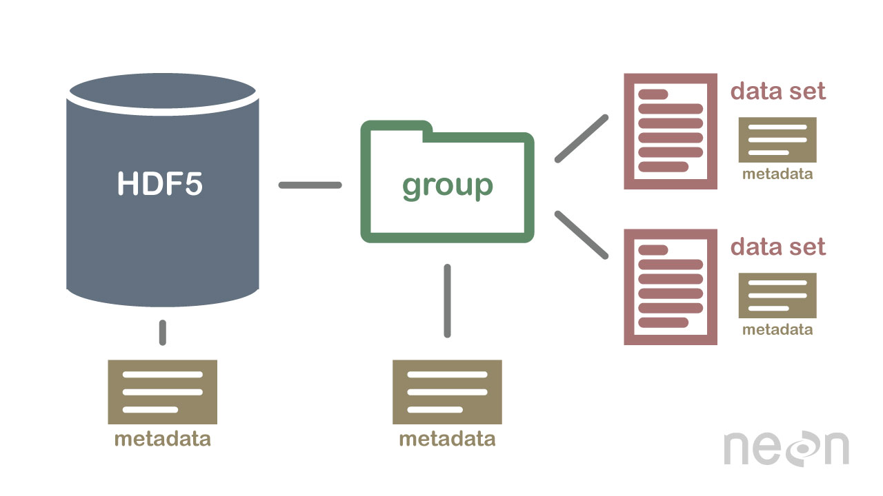**The SFTs are not always contiguous in time**, since the interferometers are not continuously online.\n\nThe typical amplitudes of the resulting signals are one or two orders of magnitude lower than the amplitude of the detector noise.\n\n\n<center>\n    <img src='https://i.imgur.com/zFflwTo.jpeg' style='width:80%; margin-left:auto; margin-right:auto' />\n    \n     Total distance: 3,027.10 km (1,880.95 mi)\n</center>\n\n\nAmong other EDAS this one includes:\n1. Bivariate histograms of frequencies and amplitude.\n2. Distributions plots per variable\n3. One dimensional Fourier Analysis\n\n\n---\nSome ideas come from previous G2Net Competitions:\n\n1. [🕳️G2Net🕳️ - EDA and Modeling](https://www.kaggle.com/code/ihelon/g2net-eda-and-modeling)\n2. [🌌 G2Net Searching the Sky: PyTorch EffNet w/ Meta](https://www.kaggle.com/code/andradaolteanu/g2net-searching-the-sky-pytorch-effnet-w-meta)\n\n\n# TOC\n\n1. [Library Import](#Library-Import)\n1. [Read Labels](#Read-Labels)\n1. [What is HDF5 and how to read it](#What-is-HDF5-and-how-to-read-it)\n1. [Ok good. Give me the pandas code](#Ok-good.-Give-me-the-pandas-code)\n1. [H1 EDA](#H1-EDA)\n    1. [H1 Spectograms](#H1-Spectograms)\n    1. [H1 Fourier Transform](#H1-Fourier-Transform)\n1. [L1 EDA](#L1-EDA)\n    1. [L1 Espectrogram](#L1-Espectrogram)\n    1. [L1 Fourier Transform](#L1-Fourier-Transform)\n1. [Distributions](#Distributions)\n    1. [Frequencies](#Frequencies)\n    1. [H1 Amplitudes](#H1-Amplitudes)\n    1. [Bivariate H1 Amplitude and Frequency](#Bivariate-H1-Amplitude-and-Frequency)\n    1. [L1 Amplitude](#L1-Amplitude)\n\n# Library Import","metadata":{}},{"cell_type":"code","source":"import pandas as pd\nimport h5py\nimport os\nimport numpy as np\nimport matplotlib.pyplot as plt\nimport matplotlib.cm as cmap\nimport matplotlib.colors as mpl_colors\nimport seaborn as sns\nimport os\n\n\ndef hex_to_rgb(h):\n    h = h.lstrip('#')\n    return tuple(int(h[i:i+2], 16)/255 for i in (0, 2, 4))\n\ncolor_palette = ['#b4d2b1', '#568f8b', '#1d4a60', '#cd7e59', '#ddb247', '#d15252']\ncolor_palette_rgb = [hex_to_rgb(x) for x in color_palette]\ncmap = mpl_colors.ListedColormap(color_palette_rgb)\ncolors = cmap.colors\nbg_color= '#fdfcf6'\n\ncustom_params = {\n    \"axes.spines.right\": False,\n    \"axes.spines.top\": False,\n    'grid.alpha':0.3,\n    'figure.figsize': (16, 6),\n    'axes.titlesize': 'Large',\n    'axes.labelsize': 'Large',\n    'figure.facecolor': bg_color,\n    'axes.facecolor': bg_color\n}\n\nsns.set_theme(\n    style='whitegrid',\n    palette=sns.color_palette(color_palette),\n    rc=custom_params\n)","metadata":{"_kg_hide-input":true,"execution":{"iopub.status.busy":"2022-10-09T18:55:16.102101Z","iopub.execute_input":"2022-10-09T18:55:16.102385Z","iopub.status.idle":"2022-10-09T18:55:16.810854Z","shell.execute_reply.started":"2022-10-09T18:55:16.102357Z","shell.execute_reply":"2022-10-09T18:55:16.809351Z"},"trusted":true},"execution_count":null,"outputs":[]},{"cell_type":"markdown","source":"# Read Labels","metadata":{}},{"cell_type":"code","source":"labels = pd.read_csv(\n    '../input/g2net-detecting-continuous-gravitational-waves/train_labels.csv',\n    names=['file', 'target'],\n    header=0,\n    index_col=0\n).squeeze()","metadata":{"execution":{"iopub.status.busy":"2022-10-09T18:55:16.812212Z","iopub.execute_input":"2022-10-09T18:55:16.812512Z","iopub.status.idle":"2022-10-09T18:55:16.831219Z","shell.execute_reply.started":"2022-10-09T18:55:16.812476Z","shell.execute_reply":"2022-10-09T18:55:16.828929Z"},"trusted":true},"execution_count":null,"outputs":[]},{"cell_type":"markdown","source":"# What is HDF5 and how to read it\n\n\n_taken from h5.py documentation_.\n\nAn HDF5 file is a container for two kinds of objects: `datasets`, which are array-like collections of data, and `groups`, which are folder-like containers that hold datasets and other groups. The most fundamental thing to remember when using h5py is:\n\n**Groups work like dictionaries, and datasets work like NumPy arrays**\n\n\n<img src='https://raw.githubusercontent.com/NEONScience/NEON-Data-Skills/dev-aten/graphics/HDF5-general/hdf5_structure2.jpg'/>\n\n\nLet's print de datasets name for the first 5 files. Apparently the dataset name is the same as the filename without extension.","metadata":{}},{"cell_type":"code","source":"# Read file\nfirst_5_files = os.listdir(\n    '../input/g2net-detecting-continuous-gravitational-waves/train/'\n)[:5]\n\nfor filename in first_5_files:\n    f = h5py.File(f'../input/g2net-detecting-continuous-gravitational-waves/train/{filename}', 'r')\n\n    # print dataset name contained in file\n    print(f'Groups in {filename}: ', list(f.keys()))","metadata":{"execution":{"iopub.status.busy":"2022-10-09T18:55:16.83474Z","iopub.execute_input":"2022-10-09T18:55:16.836441Z","iopub.status.idle":"2022-10-09T18:55:16.903319Z","shell.execute_reply.started":"2022-10-09T18:55:16.836373Z","shell.execute_reply":"2022-10-09T18:55:16.902357Z"},"trusted":true},"execution_count":null,"outputs":[]},{"cell_type":"markdown","source":"Further investigation shows that each dataset has groups 2 groups named `H1`, `L1` and one dataset named `frequency_Hz`. Both `H1` and `L1` have two datasets `SFTs` and `timestamps_GPS`\n\nThe final structure is the following:\n\n```\nGroup: 5b9f01d0f\n    |\n    |_ Group: H1\n    |    |_ Dataset: SFTs\n    |    |_ Dataset: timestamps_GPS\n    | \n    |_ Group: L1\n    |    |_ Dataset: SFTs\n    |    |_ Dataset: timestamps_GPS\n    |\n    |_ Dataset: frequency_Hz\n```","metadata":{}},{"cell_type":"code","source":"filename = '5b9f01d0f'\ndset = h5py.File(\n    f'../input/g2net-detecting-continuous-gravitational-waves/train/{filename}.hdf5', 'r'\n)[filename]\n\nprint('Groups/Datasets inisde 5b9f01d0f', dset.keys())\n\nfor group in dset.keys():\n    if isinstance(dset[group], h5py._hl.dataset.Dataset):\n        continue\n        \n    print(f'Groups inisde {group}', dset[group].keys())","metadata":{"_kg_hide-input":true,"execution":{"iopub.status.busy":"2022-10-09T18:55:16.904825Z","iopub.execute_input":"2022-10-09T18:55:16.906254Z","iopub.status.idle":"2022-10-09T18:55:16.931583Z","shell.execute_reply.started":"2022-10-09T18:55:16.906172Z","shell.execute_reply":"2022-10-09T18:55:16.930841Z"},"trusted":true},"execution_count":null,"outputs":[]},{"cell_type":"markdown","source":"# Ok good. Give me the pandas code","metadata":{"execution":{"iopub.status.busy":"2022-10-05T22:50:15.716601Z","iopub.execute_input":"2022-10-05T22:50:15.717926Z","iopub.status.idle":"2022-10-05T22:50:15.727213Z","shell.execute_reply.started":"2022-10-05T22:50:15.717871Z","shell.execute_reply":"2022-10-05T22:50:15.726039Z"}}},{"cell_type":"code","source":"def read_in_pandas(filename):\n    filename = filename[:-5]\n    \n    f = h5py.File(\n        f'../input/g2net-detecting-continuous-gravitational-waves/train/{filename}.hdf5', 'r'\n    )[filename]\n    \n    frequencies = pd.Series(\n        np.array(f['frequency_Hz']),\n        name='frequency_Hz',\n    )\n    frequencies.index = 'f_' + frequencies.index.astype(str)\n    \n    H1_timestamp_numpy = np.array(f['H1']['timestamps_GPS'], dtype=np.float32)\n    H1_timestamp = pd.Series(\n        H1_timestamp_numpy,\n        index=[f't_{i}' for i in range(len(H1_timestamp_numpy))],\n        name='h1_timestamp'\n    )\n    H1_SFTs = pd.DataFrame(\n        np.array(f['H1']['SFTs']),\n        columns=H1_timestamp.index,\n        index=frequencies\n    )\n    H1_SFTs.index.name = 'frequency'\n\n    # ---- L1\n    L1_timestamp_numpy = np.array(f['L1']['timestamps_GPS'], dtype=np.float32)\n    L1_timestamp = pd.Series(\n        L1_timestamp_numpy,\n        index=[f't_{i}' for i in range(len(L1_timestamp_numpy))],\n        name='l1_timestamp'\n    )\n    L1_SFTs = pd.DataFrame(\n        np.array(f['L1']['SFTs']),\n        columns=L1_timestamp.index,\n        index=frequencies\n    )\n    L1_SFTs.index.name = 'frequency'\n    \n    return(\n        H1_SFTs, H1_timestamp,\n        L1_SFTs, L1_timestamp,\n        frequencies\n    )\n\nH1_SFTs, H1_timestamp, L1_SFTs, L1_timestamp, frequencies = read_in_pandas('001121a05.hdf5')\nprint('Shapes:\\n')\nprint('H1_SFTs    ', H1_SFTs.shape, '   H1_timestamp', H1_timestamp.shape)\nprint('L1_SFTs    ', L1_SFTs.shape, '   L1_timestamp', L1_timestamp.shape)\nprint('Frequencies', frequencies.shape)","metadata":{"execution":{"iopub.status.busy":"2022-10-09T18:55:16.932967Z","iopub.execute_input":"2022-10-09T18:55:16.933252Z","iopub.status.idle":"2022-10-09T18:55:17.393465Z","shell.execute_reply.started":"2022-10-09T18:55:16.933227Z","shell.execute_reply":"2022-10-09T18:55:17.392482Z"},"trusted":true},"execution_count":null,"outputs":[]},{"cell_type":"markdown","source":"# H1 EDA\n\nThe first thing we notice is that not all files have the same timestamps, nor the same frequency range.\n\n> **Insights**:\n> - We could use some fixed length time-window as inputs to our models, or 1d convolutional NN\n> - Frequency is important too, my intuition is that the signal emitted by the rapidly-spinning neutron star can different amplitude in different frequencies ","metadata":{"execution":{"iopub.status.busy":"2022-10-05T23:49:32.197628Z","iopub.execute_input":"2022-10-05T23:49:32.198083Z","iopub.status.idle":"2022-10-05T23:49:32.511831Z","shell.execute_reply.started":"2022-10-05T23:49:32.198042Z","shell.execute_reply":"2022-10-05T23:49:32.510915Z"}}},{"cell_type":"code","source":"for filename in first_5_files:\n    H1_SFTs, H1_timestamp, _, _, frequencies = read_in_pandas(filename)\n    print('-'*25)\n    print(filename)\n    print('H1_SFTs     ', H1_SFTs.shape, '   H1_timestamp', H1_timestamp.shape)\n    print('Frequencies ', 'max:',frequencies.max().round(3),  '   min:',frequencies.min().round(3))\n    print()","metadata":{"execution":{"iopub.status.busy":"2022-10-09T18:55:17.395222Z","iopub.execute_input":"2022-10-09T18:55:17.395942Z","iopub.status.idle":"2022-10-09T18:55:19.045825Z","shell.execute_reply.started":"2022-10-09T18:55:17.3959Z","shell.execute_reply":"2022-10-09T18:55:19.043783Z"},"trusted":true},"execution_count":null,"outputs":[]},{"cell_type":"markdown","source":"## H1 Spectograms\n\nThis is a [good reference](#https://www.sciencedirect.com/topics/engineering/short-time-fourier-transform) to brush up concepts of signal processing.\n\n> **Insights**:\n> - Cool picture but I don't see anything different between target 1 and target 0. Maybe I need more samples.","metadata":{}},{"cell_type":"code","source":"files = [\n    #target 0 #       target 1         \n    '01bcf6533.hdf5', '001121a05.hdf5', \n    '029ed046c.hdf5', '004f23b2d.hdf5', \n    '02c8f43f3.hdf5', '00a6db666.hdf5'\n]\n\nfig, ax = plt.subplots(3, 2, figsize=(16, 15))\nax = ax.flatten()\nfor i, filename in enumerate(files):\n    H1_SFTs, H1_timestamp, _, _, frequencies = read_in_pandas(filename)\n    H1_SFTs = H1_SFTs.abs() #norm of a complex number\n    H1_SFTs.index = np.round(H1_SFTs.index, 4)\n    sns.heatmap(H1_SFTs, ax=ax[i])\n    ax[i].set_title(f'File: {filename} | Target = {i%2}', fontsize=13)\n    \nplt.tight_layout()","metadata":{"_kg_hide-input":true,"execution":{"iopub.status.busy":"2022-10-09T18:55:19.047335Z","iopub.execute_input":"2022-10-09T18:55:19.048222Z","iopub.status.idle":"2022-10-09T18:55:48.400145Z","shell.execute_reply.started":"2022-10-09T18:55:19.048192Z","shell.execute_reply":"2022-10-09T18:55:48.398829Z"},"trusted":true},"execution_count":null,"outputs":[]},{"cell_type":"markdown","source":"## H1 Fourier Transform\n\n> **Insights**:\n> - Again, cool but I don't see anything different between target 1 and target 0","metadata":{}},{"cell_type":"code","source":"files = [\n    #target 0          # target 1\n    '01bcf6533.hdf5', '001121a05.hdf5', \n    '029ed046c.hdf5', '004f23b2d.hdf5', \n    '02c8f43f3.hdf5', '00a6db666.hdf5'\n]\n\nfig, ax = plt.subplots(3, 2, figsize=(16, 15), sharey=True)\nax = ax.flatten()\nfor i, filename in enumerate(files):\n    H1_SFTs, H1_timestamp, _, _, frequencies = read_in_pandas(filename)\n    to_plot = H1_SFTs.abs().mean(axis=1)\n    ax[i].stem(to_plot.index, to_plot, linefmt=':')\n    ax[i].set_ylim(to_plot.min()*0.95, to_plot.max()*1.05)\n    ax[i].set_title(f'File: {filename} | Target = {i%2}', fontsize=13)\n    \nplt.tight_layout()","metadata":{"_kg_hide-input":true,"execution":{"iopub.status.busy":"2022-10-09T18:55:48.401479Z","iopub.execute_input":"2022-10-09T18:55:48.402036Z","iopub.status.idle":"2022-10-09T18:55:52.971576Z","shell.execute_reply.started":"2022-10-09T18:55:48.402008Z","shell.execute_reply":"2022-10-09T18:55:52.970399Z"},"trusted":true},"execution_count":null,"outputs":[]},{"cell_type":"markdown","source":"# L1 EDA\n\nFor the sake of completeness, I did the same analysis on L1 data but the results are pretty much the same than H1","metadata":{}},{"cell_type":"code","source":"for filename in first_5_files:\n    _, _, L1_SFTs, L1_timestamp, frequencies = read_in_pandas(filename)\n    print('-'*25)\n    print(filename)\n    print('L1_SFTs     ', L1_SFTs.shape, '   L1_timestamp', L1_timestamp.shape)\n    print('Frequencies ', 'max:',frequencies.max().round(3),  '   min:',frequencies.min().round(3))\n    print()","metadata":{"execution":{"iopub.status.busy":"2022-10-09T18:55:52.973165Z","iopub.execute_input":"2022-10-09T18:55:52.973479Z","iopub.status.idle":"2022-10-09T18:55:54.012145Z","shell.execute_reply.started":"2022-10-09T18:55:52.97345Z","shell.execute_reply":"2022-10-09T18:55:54.010935Z"},"trusted":true},"execution_count":null,"outputs":[]},{"cell_type":"markdown","source":"## L1 Espectrogram","metadata":{}},{"cell_type":"code","source":"files = [\n    #target 0 #       target 1         \n    '01bcf6533.hdf5', '001121a05.hdf5', \n    '029ed046c.hdf5', '004f23b2d.hdf5', \n    '02c8f43f3.hdf5', '00a6db666.hdf5'\n]\n\nfig, ax = plt.subplots(3, 2, figsize=(16, 15))\nax = ax.flatten()\nfor i, filename in enumerate(files):\n    _, _, L1_SFTs, L1_timestamp, frequencies = read_in_pandas(filename)\n    L1_SFTs = L1_SFTs.abs() # norm of a complex number\n    L1_SFTs.index = np.round(L1_SFTs.index, 4)\n    sns.heatmap(L1_SFTs, ax=ax[i])\n    ax[i].set_title(f'File: {filename} | Target = {i%2}', fontsize=13)\n    \nplt.tight_layout()","metadata":{"execution":{"iopub.status.busy":"2022-10-09T18:55:54.01347Z","iopub.execute_input":"2022-10-09T18:55:54.014222Z","iopub.status.idle":"2022-10-09T18:56:24.100789Z","shell.execute_reply.started":"2022-10-09T18:55:54.01419Z","shell.execute_reply":"2022-10-09T18:56:24.099344Z"},"trusted":true},"execution_count":null,"outputs":[]},{"cell_type":"markdown","source":"## L1 Fourier Transform","metadata":{}},{"cell_type":"code","source":"files = [\n    #target 0 #       target 1         \n    '01bcf6533.hdf5', '001121a05.hdf5', \n    '029ed046c.hdf5', '004f23b2d.hdf5', \n    '02c8f43f3.hdf5', '00a6db666.hdf5'\n]\n\nfig, ax = plt.subplots(3, 2, figsize=(16, 15), sharey=True)\nax = ax.flatten()\nfor i, filename in enumerate(files):\n    _, _, L1_SFTs, L1_timestamp, frequencies = read_in_pandas(filename)\n    L1_SFTs = L1_SFTs.abs().mean(axis=1)\n    ax[i].stem(L1_SFTs.index, to_plot, linefmt=':')\n    ax[i].set_ylim(L1_SFTs.min()*0.95, to_plot.max()*1.05)\n    ax[i].set_title(f'File: {filename} | Target = {i%2}', fontsize=13)\n    \nplt.tight_layout()","metadata":{"execution":{"iopub.status.busy":"2022-10-09T18:56:24.102097Z","iopub.execute_input":"2022-10-09T18:56:24.102351Z","iopub.status.idle":"2022-10-09T18:56:28.517417Z","shell.execute_reply.started":"2022-10-09T18:56:24.102327Z","shell.execute_reply":"2022-10-09T18:56:28.515693Z"},"trusted":true},"execution_count":null,"outputs":[]},{"cell_type":"markdown","source":"# Distributions\n\n## Frequencies\n\n> **Insights**:\n> - There is a slighty difference betwwen the distribution frequencies. Target==1 signals have more concentration in either high or low-frequencies","metadata":{}},{"cell_type":"code","source":"frequencies_list = []\nfor filename in labels[labels.ge(0)].sample(frac=0.50, random_state=0).index:\n    _, _, _, _, frequencies = read_in_pandas(filename + '.hdf5')\n    frequencies = frequencies.to_frame()\n    frequencies['target'] = labels.loc[filename]\n    frequencies_list.append(frequencies)\n    \nfrequencies = pd.concat(frequencies_list).reset_index(drop=True)\n\nfreq_bins = pd.DataFrame(\n    pd.cut(frequencies.frequency_Hz, 50, retbins=True)[1], columns=['freq_bins'])\nfreq_bins = freq_bins.astype(np.float64)\ndel frequencies_list\n\nprint(f'Using 50% of data. No frequencies: {frequencies.shape}')\n\nax = sns.kdeplot(data=frequencies, x='frequency_Hz', hue='target', common_norm=False, fill=True)\nax.grid(None)\nax.spines.left.set_visible(False)","metadata":{"_kg_hide-input":true,"execution":{"iopub.status.busy":"2022-10-09T18:56:28.521467Z","iopub.execute_input":"2022-10-09T18:56:28.522176Z","iopub.status.idle":"2022-10-09T18:57:47.876328Z","shell.execute_reply.started":"2022-10-09T18:56:28.522144Z","shell.execute_reply":"2022-10-09T18:57:47.874657Z"},"trusted":true},"execution_count":null,"outputs":[]},{"cell_type":"markdown","source":"## H1 Amplitudes\n\nI tried different seeds, and using `frac` but still the same plot.\n\n> **Insights**:\n> - Amplitude itself, is not useful.","metadata":{}},{"cell_type":"code","source":"H1_SFTs_list = []\nfor filename in labels[labels.ge(0)].sample(frac=0.05, random_state=0).index:\n    H1_SFTs, _, _, _, _ = read_in_pandas(filename + '.hdf5')\n    H1_SFTs = H1_SFTs.abs().stack().reset_index(drop=True)\n    H1_SFTs = H1_SFTs.to_frame(name='amplitude')\n    H1_SFTs['target'] = labels.loc[filename]\n    H1_SFTs_list.append(H1_SFTs)\n    \nH1_SFTs = pd.concat(H1_SFTs_list).reset_index(drop=True)\n\nH1_amplitude_bins = pd.DataFrame(\n    pd.cut(H1_SFTs.amplitude, 50, retbins=True)[1], columns=['amplitude_bins'])\nH1_amplitude_bins = H1_amplitude_bins.astype(np.float32)\ndel H1_SFTs_list\n\nprint(f'Using 5% of data. No amplitudes: {H1_SFTs.shape}')\nax = sns.histplot(data=H1_SFTs, x='amplitude', hue='target', common_norm=False, alpha=0.3)\nax.grid(None)\nax.spines.left.set_visible(False)\ndel H1_SFTs","metadata":{"_kg_hide-input":true,"execution":{"iopub.status.busy":"2022-10-09T18:57:47.877751Z","iopub.execute_input":"2022-10-09T18:57:47.878069Z","iopub.status.idle":"2022-10-09T18:58:33.773454Z","shell.execute_reply.started":"2022-10-09T18:57:47.878021Z","shell.execute_reply":"2022-10-09T18:58:33.771351Z"},"trusted":true},"execution_count":null,"outputs":[]},{"cell_type":"markdown","source":"## Bivariate H1 Amplitude and Frequency\n\nI can process 100% with a minimum footprint on RAM to produce a bi-variate histogram using cumulative counts from some pre-fitted bins and processing one file at a time.  It is a great trick to visualize the entire dataset in one picture, at the expense of the time taken to read each file.\n\n> **Insights**:\n> - Same as plotting only frequency on a one-dimensional plot.","metadata":{"execution":{"iopub.status.busy":"2022-10-06T02:39:23.470568Z","iopub.execute_input":"2022-10-06T02:39:23.471008Z","iopub.status.idle":"2022-10-06T02:39:23.484904Z","shell.execute_reply.started":"2022-10-06T02:39:23.470974Z","shell.execute_reply":"2022-10-06T02:39:23.483486Z"}}},{"cell_type":"code","source":"%%time\nH1_SFTs_list = []\nfor filename in labels[labels.ge(0)].index:\n    H1_SFTs, _, _, _, _ = read_in_pandas(filename + '.hdf5')\n    H1_SFTs = H1_SFTs.abs().stack().reset_index().drop(columns='level_1')\n    H1_SFTs.columns = ['frequency', 'amplitude']\n    H1_SFTs['target'] = labels.loc[filename]\n    \n    H1_SFTs = pd.merge_asof(\n        H1_SFTs.sort_values('frequency'), freq_bins, left_on='frequency', right_on='freq_bins')\n    H1_SFTs = pd.merge_asof(\n        H1_SFTs.sort_values('amplitude'), H1_amplitude_bins, left_on='amplitude', right_on='amplitude_bins')\n    H1_SFTs_list.append(\n        H1_SFTs.groupby([\n            'target', 'freq_bins', 'amplitude_bins'\n        ]).size())\n    \nH1_SFTs = pd.concat(H1_SFTs_list).groupby(level=[0, 1, 2]).sum()\ndel H1_SFTs_list\n\nfig, ax = plt.subplots(2, 1, figsize=(16, 10))\nfor target in [0, 1]:\n    sns.heatmap(H1_SFTs.unstack(level=1).xs(target, level=0), ax=ax[target])\n    ax[target].set_title(f'Target == {target}')\n    ax[target].xaxis.set_major_formatter('{:.2e}'.format)\n    ax[target].yaxis.set_major_formatter('{:.2e}'.format)\n    \nplt.tight_layout()","metadata":{"_kg_hide-input":true,"execution":{"iopub.status.busy":"2022-10-09T18:58:33.774747Z","iopub.execute_input":"2022-10-09T18:58:33.776146Z","iopub.status.idle":"2022-10-09T19:10:36.620385Z","shell.execute_reply.started":"2022-10-09T18:58:33.776113Z","shell.execute_reply":"2022-10-09T19:10:36.619204Z"},"trusted":true},"execution_count":null,"outputs":[]},{"cell_type":"markdown","source":"## L1 Amplitude\n\n> **Insights**:\n> - Same as before, amplitude itself, is not useful.","metadata":{"execution":{"iopub.status.busy":"2022-10-06T03:51:01.442229Z","iopub.execute_input":"2022-10-06T03:51:01.443288Z"}}},{"cell_type":"code","source":"L1_SFTs_list = []\nfor filename in labels[labels.ge(0)].sample(frac=0.05, random_state=0).index:\n    _, _, L1_SFTs, _, _ = read_in_pandas(filename + '.hdf5')\n    L1_SFTs = L1_SFTs.abs().stack().reset_index(drop=True)\n    L1_SFTs = L1_SFTs.to_frame(name='amplitude')\n    L1_SFTs['target'] = labels.loc[filename]\n    L1_SFTs_list.append(L1_SFTs)\n    \n\nL1_SFTs = pd.concat(L1_SFTs_list).reset_index(drop=True)\nL1_amplitude_bins = pd.DataFrame(\n    pd.cut(L1_SFTs.amplitude, 50, retbins=True)[1], columns=['amplitude_bins'])\nL1_amplitude_bins = L1_amplitude_bins.astype(np.float32)\ndel L1_SFTs_list\n\nprint(f'Using 5% of data. No amplitudes: {L1_SFTs.shape}')\n\nax = sns.kdeplot(data=L1_SFTs, x='amplitude', hue='target', common_norm=False, fill=True)\nax.grid(None)\nax.spines.left.set_visible(False)\ndel L1_SFTs","metadata":{"execution":{"iopub.status.busy":"2022-10-09T19:10:36.621866Z","iopub.execute_input":"2022-10-09T19:10:36.622756Z","iopub.status.idle":"2022-10-09T19:15:13.376714Z","shell.execute_reply.started":"2022-10-09T19:10:36.622722Z","shell.execute_reply":"2022-10-09T19:15:13.374761Z"},"trusted":true},"execution_count":null,"outputs":[]},{"cell_type":"markdown","source":"## Bivariate L1 Amplitude and Frequency\n\n> **Insights**:\n> - Same as plotting only frequency on a one-dimensional plot.","metadata":{}},{"cell_type":"code","source":"%%time\nL1_SFTs_list = []\nfor filename in labels[labels.ge(0)].index:\n    _, _, L1_SFTs, _, _ = read_in_pandas(filename + '.hdf5')\n    L1_SFTs = L1_SFTs.abs().stack().reset_index().drop(columns='level_1')\n    L1_SFTs.columns = ['frequency', 'amplitude']\n    L1_SFTs['target'] = labels.loc[filename]\n    \n    L1_SFTs = pd.merge_asof(\n        L1_SFTs.sort_values('frequency'), freq_bins, left_on='frequency', right_on='freq_bins')\n    L1_SFTs = pd.merge_asof(\n        L1_SFTs.sort_values('amplitude'), L1_amplitude_bins, left_on='amplitude', right_on='amplitude_bins')\n    L1_SFTs_list.append(\n        L1_SFTs.groupby([\n            'target', 'freq_bins', 'amplitude_bins'\n        ]).size())\n    \nL1_SFTs = pd.concat(L1_SFTs_list).groupby(level=[0, 1, 2]).sum()\ndel L1_SFTs_list\n\nfig, ax = plt.subplots(2, 1, figsize=(16, 10))\nfor target in [0, 1]:\n    sns.heatmap(L1_SFTs.unstack(level=1).xs(target, level=0), ax=ax[target])\n    ax[target].set_title(f'Target == {target}')\n    ax[target].xaxis.set_major_formatter('{:.2e}'.format)\n    ax[target].yaxis.set_major_formatter('{:.2e}'.format)\n    \nplt.tight_layout()","metadata":{"execution":{"iopub.status.busy":"2022-10-09T19:15:13.379629Z","iopub.execute_input":"2022-10-09T19:15:13.380107Z","iopub.status.idle":"2022-10-09T19:27:17.29681Z","shell.execute_reply.started":"2022-10-09T19:15:13.380068Z","shell.execute_reply":"2022-10-09T19:27:17.295518Z"},"trusted":true},"execution_count":null,"outputs":[]}]}