
\n(figure from this arxiv.org/abs/2206.06447)
We want to thank the organizers and the other participants of this great event! This is our first time on Kaggle and we are happy to win the Gold medal.
\nWe are theoretical particle physicists working mainly on Heavy Neutral Leptons (hence the team name with the same acronym) with no background in Gravitational Wave physics. The initial plan was to improve our ML skills, but we turned eventually to a physics-based approach.
\nIt is easy to find a continuous signal – it is just a peak in a Fourier transform.
\nHowever, due to the Doppler modulation and spin-down of the neutron star, the signal is spread over multiple frequency bins.
\nOur method (very similar to Jun Koda's solution) aims to streamline the modulation curve, as in the figure below
\n(figure from this arxiv.org/abs/2206.06447)
The modulation pattern depends on the position of the source (alpha, delta) and the time derivative of the frequency F1, see the pyFstat tutorial.
\nIn fact, the method is not new and has been used by the GW community under the name of StaSlide [1]. Once the individual SFTs are shifted so that the signal is located in one frequency bin, we simply sum their powers (absolute values squared). If the modulation pattern mismatches the actual one slightly, the signal is spread across several bins which drastically reduces the sensitivity. Therefore, one has to scan over a very fine grid in the parameter space. The method is insensitive to any gaps in the timestamps. It is also rather robust against non-stationary noise, but very sensitive to instrumental lines.
\nFor this challenge, we have implemented the method from scratch, first in python and then in Julia (the optimized Julia code gives a ~240x speed-up compared to a naive python implementation).
\nThe processing followed these steps:
\nProcessing the test set takes around 10 hours on a 5-year-old Linux desktop machine (on 8 cores).
\nLike a good Kaggle beginner, we initially jumped at the most high-tech solution possible: we wanted to use a Transformer applied to time series. We realized that there is an existing method to search for CWs that generates sequential data: Viterbi tracks [2].
\nAfter this attempt failed, we then decided to temper our expectations and go for a known and tested method: convolutional neural networks (in particular we searched for noise-resilient CNNs). Here we encountered a number of problems. First, the timestamps are not nicely aligned on a grid, and the SFTs contain a large number of gaps and overlaps. The number of timesteps is also too large to feed into a typical CNN architecture. We realized that we would need to resize our input, and we tried to find a clever way to do so, that didn’t penalize our sensitivity too much (having worked previously on resonant particle searches, we were all well-aware of the importance of maintaining the best possible resolution). To this end we tried a number of filters to match the daily amplitude and frequency modulations before max-pooling the SFTs for each day.
\nWe had limited success here: we managed to make some hidden CWs much more visible to the human eye, but when we tried to use this method to produce the CNN input, we encountered a much bigger problem: the test set was significantly out-of-distribution compared to the training set, with a number of test samples containing strong glitches (see for instance these posts and this notebook). We realized that we would need to generate our own training set if we wanted to apply any machine learning method. This gave us the impetus to look at algorithmic methods that do not require a training set.
\nWe also tried more elaborate methods of normalizing data, like the rolling median normalization, but it didn’t improve our results and seemingly increased the look-elsewhere effect.
\nWe want to thank the organizers and the other participants of this great event! This is our first time on Kaggle and we are happy to win the Gold medal.
\nWe are theoretical particle physicists working mainly on Heavy Neutral Leptons (hence the team name with the same acronym) with no background in Gravitational Wave physics. The initial plan was to improve our ML skills, but we turned eventually to a physics-based approach.
\nIt is easy to find a continuous signal – it is just a peak in a Fourier transform.
\nHowever, due to the Doppler modulation and spin-down of the neutron star, the signal is spread over multiple frequency bins.
\nOur method (very similar to Jun Koda's solution) aims to streamline the modulation curve, as in the figure below
\n(figure from this arxiv.org/abs/2206.06447)
The modulation pattern depends on the position of the source (alpha, delta) and the time derivative of the frequency F1, see the pyFstat tutorial.
\nIn fact, the method is not new and has been used by the GW community under the name of StaSlide [1]. Once the individual SFTs are shifted so that the signal is located in one frequency bin, we simply sum their powers (absolute values squared). If the modulation pattern mismatches the actual one slightly, the signal is spread across several bins which drastically reduces the sensitivity. Therefore, one has to scan over a very fine grid in the parameter space. The method is insensitive to any gaps in the timestamps. It is also rather robust against non-stationary noise, but very sensitive to instrumental lines.
\nFor this challenge, we have implemented the method from scratch, first in python and then in Julia (the optimized Julia code gives a ~240x speed-up compared to a naive python implementation).
\nThe processing followed these steps:
\nProcessing the test set takes around 10 hours on a 5-year-old Linux desktop machine (on 8 cores).
\nLike a good Kaggle beginner, we initially jumped at the most high-tech solution possible: we wanted to use a Transformer applied to time series. We realized that there is an existing method to search for CWs that generates sequential data: Viterbi tracks [2].
\nAfter this attempt failed, we then decided to temper our expectations and go for a known and tested method: convolutional neural networks (in particular we searched for noise-resilient CNNs). Here we encountered a number of problems. First, the timestamps are not nicely aligned on a grid, and the SFTs contain a large number of gaps and overlaps. The number of timesteps is also too large to feed into a typical CNN architecture. We realized that we would need to resize our input, and we tried to find a clever way to do so, that didn’t penalize our sensitivity too much (having worked previously on resonant particle searches, we were all well-aware of the importance of maintaining the best possible resolution). To this end we tried a number of filters to match the daily amplitude and frequency modulations before max-pooling the SFTs for each day.
\nWe had limited success here: we managed to make some hidden CWs much more visible to the human eye, but when we tried to use this method to produce the CNN input, we encountered a much bigger problem: the test set was significantly out-of-distribution compared to the training set, with a number of test samples containing strong glitches (see for instance these posts and this notebook). We realized that we would need to generate our own training set if we wanted to apply any machine learning method. This gave us the impetus to look at algorithmic methods that do not require a training set.
\nWe also tried more elaborate methods of normalizing data, like the rolling median normalization, but it didn’t improve our results and seemingly increased the look-elsewhere effect.
\nWhoa, another method to solve the problem. Very cool.
", "rawMarkdown": "Whoa, another method to solve the problem. Very cool.", "votes": 1, "replies": [ { "id": 2087344, "postDate": "2023-01-05T14:38:09.420Z", "content": "Thank you!
", "rawMarkdown": "Thank you!", "votes": 1 } ] }, { "id": 2100816, "postDate": "2023-01-15T12:56:50.070Z", "content": "Congratulations! Your trials with both Julia and Python were amazing. The differential evolution method helped me grasp another method for noise reduction, other than t-test validation.
", "rawMarkdown": "Congratulations! Your trials with both Julia and Python were amazing. The differential evolution method helped me grasp another method for noise reduction, other than t-test validation.", "replies": [ { "id": 2101885, "postDate": "2023-01-16T09:00:22.327Z", "content": "Great, happy to hear that!
", "rawMarkdown": "Great, happy to hear that!" } ] }, { "id": 2086819, "postDate": "2023-01-05T04:20:29.743Z", "content": "have you guys opensource your Julia code? Would love to read/share it :)
", "rawMarkdown": "have you guys opensource your Julia code? Would love to read/share it :)", "replies": [ { "id": 2087348, "postDate": "2023-01-05T14:39:57.503Z", "content": "Yes, we are planning to open source it and maybe writing a more detailed post. It will take some time to cleanup the code though.
", "rawMarkdown": "Yes, we are planning to open source it and maybe writing a more detailed post. It will take some time to cleanup the code though.", "votes": 2, "replies": [ { "id": 2087419, "postDate": "2023-01-05T15:28:58.570Z", "content": "How can I follow up? Will you comment the blog like here? Are you on twitter? I don't want to miss it once it's live
", "rawMarkdown": "How can I follow up? Will you comment the blog like here? Are you on twitter? I don't want to miss it once it's live " }, { "id": 2101889, "postDate": "2023-01-16T09:03:47.110Z", "content": "Sorry for late reply, we still haven't prepared the repository. We will post it here for sure. I have a twitter account: https://twitter.com/ITimiryasov, maybe I need to start twitting :)
", "rawMarkdown": "Sorry for late reply, we still haven't prepared the repository. We will post it here for sure. I have a twitter account: https://twitter.com/ITimiryasov, maybe I need to start twitting :) " } ] } ] } ], "comments": [ { "id": 2085955, "author_name": "DennisSakva", "author_url": "", "post_date": "2023-01-04T13:36:14.733000", "content": "Whoa, another method to solve the problem. Very cool.
", "votes": 1, "replies": [ { "id": 2087344, "author_name": "Inar Timiryasov", "author_url": "", "post_date": "2023-01-05T14:38:09.420000", "content": "Thank you!
", "votes": 1, "replies": [] } ] }, { "id": 2100816, "author_name": "Suma Mallapragada", "author_url": "", "post_date": "2023-01-15T12:56:50.070000", "content": "Congratulations! Your trials with both Julia and Python were amazing. The differential evolution method helped me grasp another method for noise reduction, other than t-test validation.
", "votes": 0, "replies": [ { "id": 2101885, "author_name": "Inar Timiryasov", "author_url": "", "post_date": "2023-01-16T09:00:22.327000", "content": "Great, happy to hear that!
", "votes": 0, "replies": [] } ] }, { "id": 2086819, "author_name": "Abhimanyu Aryan", "author_url": "", "post_date": "2023-01-05T04:20:29.743000", "content": "have you guys opensource your Julia code? Would love to read/share it :)
", "votes": 0, "replies": [ { "id": 2087348, "author_name": "Inar Timiryasov", "author_url": "", "post_date": "2023-01-05T14:39:57.503000", "content": "Yes, we are planning to open source it and maybe writing a more detailed post. It will take some time to cleanup the code though.
", "votes": 2, "replies": [ { "id": 2087419, "author_name": "Abhimanyu Aryan", "author_url": "", "post_date": "2023-01-05T15:28:58.570000", "content": "How can I follow up? Will you comment the blog like here? Are you on twitter? I don't want to miss it once it's live
", "votes": 0, "replies": [] }, { "id": 2101889, "author_name": "Inar Timiryasov", "author_url": "", "post_date": "2023-01-16T09:03:47.110000", "content": "Sorry for late reply, we still haven't prepared the repository. We will post it here for sure. I have a twitter account: https://twitter.com/ITimiryasov, maybe I need to start twitting :)
", "votes": 0, "replies": [] } ] } ] } ], "raw_markdown_by_id": { "2085890": "We want to thank the organizers and the other participants of this great event! This is our first time on Kaggle and we are happy to win the Gold medal.\n\nWe are theoretical particle physicists working mainly on Heavy Neutral Leptons (hence the team name with the same acronym) with no background in Gravitational Wave physics. The initial plan was to improve our ML skills, but we turned eventually to a physics-based approach.\n\n\n\n## The idea of the Method\n\nIt is easy to find a continuous signal – it is just a peak in a Fourier transform.\nHowever, due to the Doppler modulation and spin-down of the neutron star, the signal is spread over multiple frequency bins. \nOur method (very similar to Jun Koda's solution) aims to streamline the modulation curve, as in the figure below \n\n\n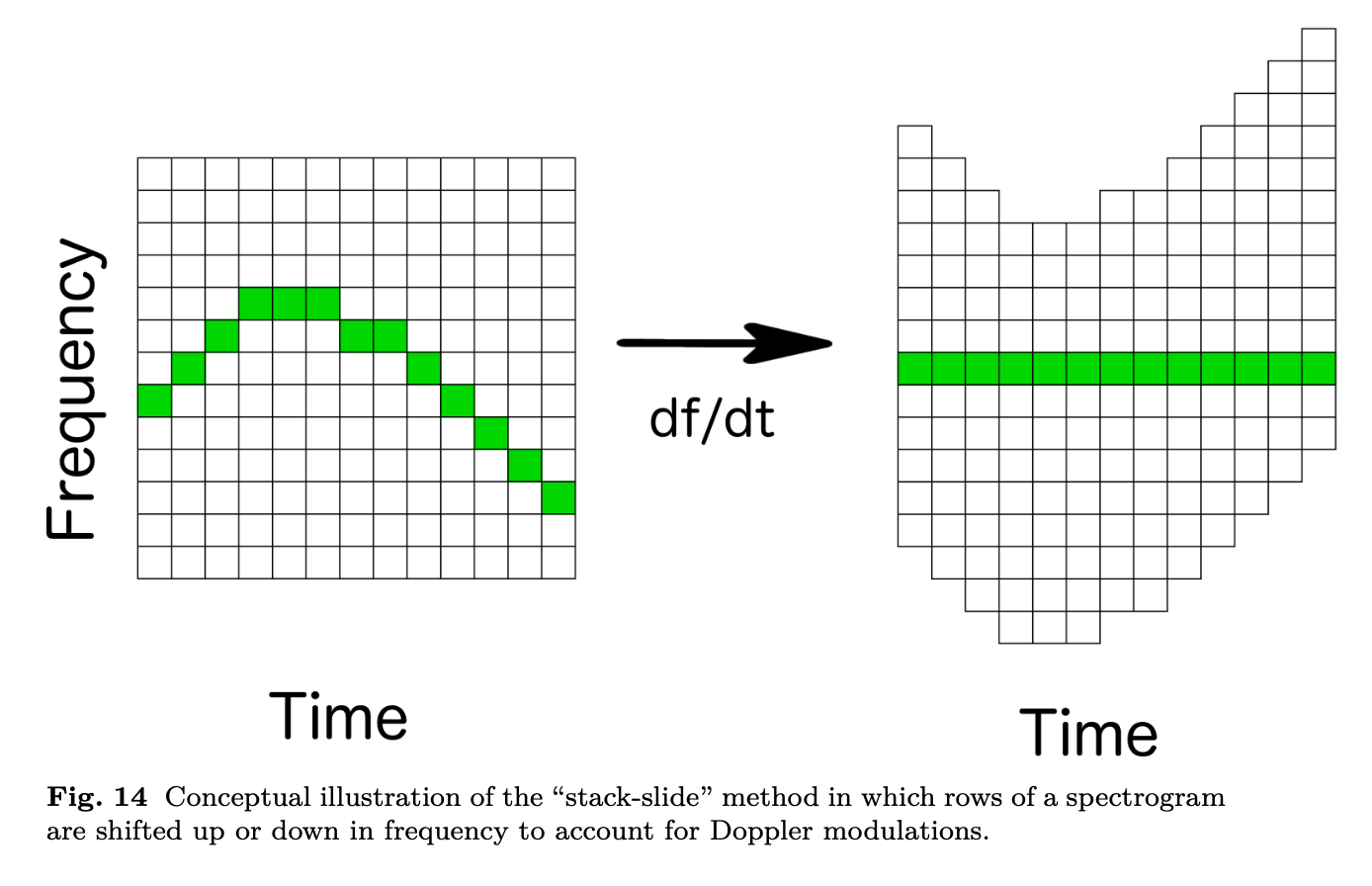\n(figure from this [arxiv.org/abs/2206.06447](https://arxiv.org/abs/2206.06447.))\n\nThe modulation pattern depends on the position of the source (alpha, delta) and the time derivative of the frequency F1, see the [pyFstat tutorial](https://github.com/PyFstat/PyFstat/blob/master/examples/tutorials/1_generating_signals.ipynb).\n\nIn fact, the method is not new and has been used by the GW community under the name of StaSlide [1]. Once the individual SFTs are shifted so that the signal is located in one frequency bin, we simply sum their powers (absolute values squared). If the modulation pattern mismatches the actual one slightly, the signal is spread across several bins which drastically reduces the sensitivity. Therefore, one has to scan over a very fine grid in the parameter space. The method is insensitive to any gaps in the timestamps. It is also rather robust against non-stationary noise, but very sensitive to instrumental lines.\n\n\n## Implementation\n\nFor this challenge, we have implemented the method from scratch, first in python and then in Julia (the optimized Julia code gives a ~240x speed-up compared to a naive python implementation).\n\nThe processing followed these steps:\n* Normalize the data. |SFT|² / std(Re(SFT)) worked just well. We tweaked this a bit when a strong instrumental line was detected by the algorithm, but it didn’t seem to affect the performance. Normalized this way, the gaussian noise will follow chi2 distribution and the signal will follow non-central chi2. \n* For every sample, scan over the parameter space (alpha, delta, f1) and find the maximum power. Scanning over alpha and delta with sufficient resolution takes ~20 s per sample, so scanning over f1 was too time-consuming for us. So we used [differential](https://github.com/robertfeldt/BlackBoxOptim.jl) [evolution](https://en.wikipedia.org/wiki/Differential_evolution) with the objective - max ( Power_L1 + Power_H1). Summing the powers from two detectors greatly improved our LB (from 0.747 to 0.804).\n* During the scan, our algorithm analyzed the data to isolate potential glitches. Improving this algorithm slightly improved our score.\n* Final predictions were made by simply applying the logistic function to the max Power. AUC score is invariant under reparametrization, so the parameters of the logistic function do not matter.\n\nProcessing the test set takes around 10 hours on a 5-year-old Linux desktop machine (on 8 cores).\n\n\n\n## What could have been improved\n\n* Amplitude modulation. The signal intensity depends on the position of the detectors compared to the source, and an extra phase in a complicated way. We wanted to sum the stacks with weights proportional to that amplitude modulation but didn’t have time to implement that properly. If we understand correctly, Jun Kodo used amplitude modulation. Simpler filters (daily/twice-daily modulation \\\\( \\propto \\exp(2πi t/T) \\\\)) did not perform well.\n* Maybe we concentrated too much on isolating glitches, which make up at most 2% of the test set.\n* Optimal filtering. We noticed the signal leakage to the nearby frequency bins due to the finite time of short SFTs. Mitigating it with optimal filtering is a great idea, which put Jun Kodo in the 1st place. We initially tried to filter the SFTs when investigating the use of CNNs, however, we did not have time to revive this effort for stack-sliding.\n\n\n## Earlier failed attempts\n\nLike a good Kaggle beginner, we initially jumped at the most high-tech solution possible: we wanted to use a Transformer applied to time series. We realized that there is an existing method to search for CWs that generates sequential data: Viterbi tracks [2].\n\nAfter this attempt failed, we then decided to temper our expectations and go for a known and tested method: convolutional neural networks (in particular we searched for noise-resilient CNNs). Here we encountered a number of problems. First, the timestamps are not nicely aligned on a grid, and the SFTs contain a large number of gaps and overlaps. The number of timesteps is also too large to feed into a typical CNN architecture. We realized that we would need to resize our input, and we tried to find a clever way to do so, that didn’t penalize our sensitivity too much (having worked previously on resonant particle searches, we were all well-aware of the importance of maintaining the best possible resolution). To this end we tried a number of filters to match the daily amplitude and frequency modulations before max-pooling the SFTs for each day.\n\nWe had limited success here: we managed to make some hidden CWs much more visible to the human eye, but when we tried to use this method to produce the CNN input, we encountered a much bigger problem: the test set was significantly out-of-distribution compared to the training set, with a number of test samples containing strong glitches (see for instance [these](https://www.kaggle.com/competitions/g2net-detecting-continuous-gravitational-waves/discussion/364854#2026621) [posts](https://www.kaggle.com/competitions/g2net-detecting-continuous-gravitational-waves/discussion/364854#2022856) and [this notebook](https://www.kaggle.com/code/vslaykovsky/g2net-winning-strategy-with-external-data)). We realized that we would need to generate our own training set if we wanted to apply any machine learning method. This gave us the impetus to look at algorithmic methods that do not require a training set.\n\nWe also tried more elaborate methods of normalizing data, like the rolling median normalization, but it didn’t improve our results and seemingly increased the look-elsewhere effect. \n\n\n\n## References\n\n1. LIGO Scientific Collaboration, *All-sky search for periodic gravitational waves in LIGO S4 data,* Phys.Rev.D 77 (2008) 022001, Phys.Rev.D 80 (2009) 129904 (erratum), [arXiv:0708.3818](https://arxiv.org/abs/0708.3818)\n2. Joe Bayley, Graham Woan, Chris Messenger, *Generalized application of the Viterbi algorithm to searches for continuous gravitational-wave signals,* Phys.Rev.D 100 (2019) 2, 023006, [arXiv:1903.12614](https://arxiv.org/abs/1903.12614)", "2085955": "Whoa, another method to solve the problem. Very cool.", "2100816": "Congratulations! Your trials with both Julia and Python were amazing. The differential evolution method helped me grasp another method for noise reduction, other than t-test validation.", "2086819": "have you guys opensource your Julia code? Would love to read/share it :)" } }