
Many thanks to the organizers and to Kaggle for hosting this very interesting competion! We also thank all competitors for the discussions and the exchange of ideas. We learned a lot about CW physics and spectra processing. We are sorry that we did not use a machine learning method. We actually tried but our little experience did not lead to anything satisfying :-)
\nWe quickly found different ways to generate solutions and looked for the best way to ensemble them. But we haven't found an obvious way with the AUC ROC function ranking paradigm. Our idea then was to have a single judge function to evaluate homogeneously all the methods. Each method tried to determine the position of the CW curve in SFT, defined by 4 parameters (F0, F1, alpha, delta). Then, the judge function kept, for each test case, the parameters leading to the best metric score among all results.
\nThus, we have accumulated the results of a few methods executed with different numerical parameters. It is interesting to notice that the best contributions were distributed among the various methods. A disadvantage of this judge function was that it required all participating methods to be able to provide the position of the CW curve with all four parameters.
\nCW parameters generators
\nA set of algorithms are run on each test case to try to find candidate CW parameters for the potential signal present in the spectrogram. They differ mainly in the processing blocks variants and their parameterization. The main steps were:
Coarse estimator (dynamic programming)
\nNormalized L1 and H1 spectrograms are merged: abs(SFT_H1)² + abs(SFT_L1)²
\nOn some variants, non-stationary noise correction is applied to reduce the impact of artifacts.
\nA frequency densification x2 or x4 is also optionally considered (e.g. sft[1::2, :] = (sft_[:-1, :] - sft_[1:, :]) / np.sqrt(2) on the complex SFTs for the x2 version).
Two main dynamic programming variants were considered, gradually building the best curve with increasing time step:
\n1) Horizontal binning
\nIn this variant the spectrogram is binned horizontally over each timestep and the curve is allowed to go up or down up to one frequency bin per timestep. Only one inflexion point is allowed.
2) Restricted slope variations
\nIn this variant the signal is interpolated along segments with fixed slopes. The slope range is determined by the maximum expected doppler for the frequency band and by the f1-range considered, and the slope variations between two time steps are clamped. Only one inflexion point is also allowed.
Parameters estimation
\nA parametric fit of the curve obtained with the previous step gives us an approximate curve in the form (f0 + f1 * t) * (1 + A * cos(phi + w * t))
\nw corresponds to the mean motion of the Earth in an intertial frame, and A is limited to taking into account its maximal inertial velocity.
\nThen two possible alternative source positions (on each side of the ecliptic) are derived from these intermediate A and phi parameters.
Parameters optimization
\nWe then try to optimize these sets of (f0, f1, alpha, delta) CW parameters with a Nelder-Mead algorithm.
\nAt this step we go back to the original complex L1 and H1 SFTs. As illustrated in more detail in the next section, the signal is integrated independently for both detectors along the parametric curves, and the minimum value min(L1, H1) is considered for the optimization. A simplified interpolation is performed in the complex SFTs considering only 2 enclosing points in place of the full vector considered in the judge. With a cos i = 1 assumption, an amplitude ponderation is applied along the time axis during the signal integration, and an optional weighting is applied to cope with noise artifacts.
\nOnly the best of the two possible source directions is kept after this step.
Signal strength evaluation (\"judge\")
\nThe judge evaluation works on the raw complex spectra H1 and L1. We wanted to determine a SNR on both indenpendently. Note that what we call SNR is probably quite different of the definition one can find in PyFstat.
Here are the main steps of the judge algorithm :
\nFor every time slot (spectrum column):
\nSum the square modulus obtained for each time slot (weighted by the inverse variance of the columns, and by the amplitude modulation expected for a cos i = 1 signal).
\nWe determined empirically (on public score) that the best metric to keep was min(SNR_H1, SNR_L1), but the sum SNR_H1 + SNR_L1 performed better on the train dataset. Also, 2 * min(SNR_H1, SNR_L1) + max(SNR_H1, SNR_L1) seems to have an important positive gap on the private dataset (our best submission so far scores 0.821 on private but we did not keep it as it was scoring 0.807 on public score).
\nWe noticed that the scores of the high frequency spectra were significantly lower in average. Our research method probably performed worse on it due to the daily Doppler implying a 1-pixel frequency variation. Applying a score correction of the linear regression made us gain between 0.002 and 0.005 points on submissions.
\nThanks again to everyone for this journey. We are impressed by the diversity of the various methods used to tackle this problem :-)
", "messages": [ { "id": 2087842, "postDate": "2023-01-05T20:57:40.110Z", "content": "Many thanks to the organizers and to Kaggle for hosting this very interesting competion! We also thank all competitors for the discussions and the exchange of ideas. We learned a lot about CW physics and spectra processing. We are sorry that we did not use a machine learning method. We actually tried but our little experience did not lead to anything satisfying :-)
\nWe quickly found different ways to generate solutions and looked for the best way to ensemble them. But we haven't found an obvious way with the AUC ROC function ranking paradigm. Our idea then was to have a single judge function to evaluate homogeneously all the methods. Each method tried to determine the position of the CW curve in SFT, defined by 4 parameters (F0, F1, alpha, delta). Then, the judge function kept, for each test case, the parameters leading to the best metric score among all results.
\nThus, we have accumulated the results of a few methods executed with different numerical parameters. It is interesting to notice that the best contributions were distributed among the various methods. A disadvantage of this judge function was that it required all participating methods to be able to provide the position of the CW curve with all four parameters.
\nCW parameters generators
\nA set of algorithms are run on each test case to try to find candidate CW parameters for the potential signal present in the spectrogram. They differ mainly in the processing blocks variants and their parameterization. The main steps were:
Coarse estimator (dynamic programming)
\nNormalized L1 and H1 spectrograms are merged: abs(SFT_H1)² + abs(SFT_L1)²
\nOn some variants, non-stationary noise correction is applied to reduce the impact of artifacts.
\nA frequency densification x2 or x4 is also optionally considered (e.g. sft[1::2, :] = (sft_[:-1, :] - sft_[1:, :]) / np.sqrt(2) on the complex SFTs for the x2 version).
Two main dynamic programming variants were considered, gradually building the best curve with increasing time step:
\n1) Horizontal binning
\nIn this variant the spectrogram is binned horizontally over each timestep and the curve is allowed to go up or down up to one frequency bin per timestep. Only one inflexion point is allowed.
2) Restricted slope variations
\nIn this variant the signal is interpolated along segments with fixed slopes. The slope range is determined by the maximum expected doppler for the frequency band and by the f1-range considered, and the slope variations between two time steps are clamped. Only one inflexion point is also allowed.
Parameters estimation
\nA parametric fit of the curve obtained with the previous step gives us an approximate curve in the form (f0 + f1 * t) * (1 + A * cos(phi + w * t))
\nw corresponds to the mean motion of the Earth in an intertial frame, and A is limited to taking into account its maximal inertial velocity.
\nThen two possible alternative source positions (on each side of the ecliptic) are derived from these intermediate A and phi parameters.
Parameters optimization
\nWe then try to optimize these sets of (f0, f1, alpha, delta) CW parameters with a Nelder-Mead algorithm.
\nAt this step we go back to the original complex L1 and H1 SFTs. As illustrated in more detail in the next section, the signal is integrated independently for both detectors along the parametric curves, and the minimum value min(L1, H1) is considered for the optimization. A simplified interpolation is performed in the complex SFTs considering only 2 enclosing points in place of the full vector considered in the judge. With a cos i = 1 assumption, an amplitude ponderation is applied along the time axis during the signal integration, and an optional weighting is applied to cope with noise artifacts.
\nOnly the best of the two possible source directions is kept after this step.
Signal strength evaluation (\"judge\")
\nThe judge evaluation works on the raw complex spectra H1 and L1. We wanted to determine a SNR on both indenpendently. Note that what we call SNR is probably quite different of the definition one can find in PyFstat.
Here are the main steps of the judge algorithm :
\nFor every time slot (spectrum column):
\nSum the square modulus obtained for each time slot (weighted by the inverse variance of the columns, and by the amplitude modulation expected for a cos i = 1 signal).
\nWe determined empirically (on public score) that the best metric to keep was min(SNR_H1, SNR_L1), but the sum SNR_H1 + SNR_L1 performed better on the train dataset. Also, 2 * min(SNR_H1, SNR_L1) + max(SNR_H1, SNR_L1) seems to have an important positive gap on the private dataset (our best submission so far scores 0.821 on private but we did not keep it as it was scoring 0.807 on public score).
\nWe noticed that the scores of the high frequency spectra were significantly lower in average. Our research method probably performed worse on it due to the daily Doppler implying a 1-pixel frequency variation. Applying a score correction of the linear regression made us gain between 0.002 and 0.005 points on submissions.
\nThanks again to everyone for this journey. We are impressed by the diversity of the various methods used to tackle this problem :-)
", "rawMarkdown": "Many thanks to the organizers and to Kaggle for hosting this very interesting competion! We also thank all competitors for the discussions and the exchange of ideas. We learned a lot about CW physics and spectra processing. We are sorry that we did not use a machine learning method. We actually tried but our little experience did not lead to anything satisfying :-)\n\nWe quickly found different ways to generate solutions and looked for the best way to ensemble them. But we haven't found an obvious way with the AUC ROC function ranking paradigm. Our idea then was to have a single judge function to evaluate homogeneously all the methods. Each method tried to determine the position of the CW curve in SFT, defined by 4 parameters (F0, F1, alpha, delta). Then, the judge function kept, for each test case, the parameters leading to the best metric score among all results.\n\nThus, we have accumulated the results of a few methods executed with different numerical parameters. It is interesting to notice that the best contributions were distributed among the various methods. A disadvantage of this judge function was that it required all participating methods to be able to provide the position of the CW curve with all four parameters.\n\n**CW parameters generators**\nA set of algorithms are run on each test case to try to find candidate CW parameters for the potential signal present in the spectrogram. They differ mainly in the processing blocks variants and their parameterization. The main steps were:\n\n- first use dynamic programming to sketch a rough estimate of the signal curve,\n- then infer the approximate associated CW parameters (f0, f1, and source direction),\n- finally adjust the parameters to the signal with an optimisation algorithm (we used the Nelder-Mead optimizer of scipy).\n\n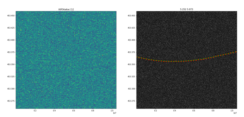\n\n**Coarse estimator (dynamic programming)**\nNormalized L1 and H1 spectrograms are merged: abs(SFT_H1)² + abs(SFT_L1)²\nOn some variants, non-stationary noise correction is applied to reduce the impact of artifacts.\nA frequency densification x2 or x4 is also optionally considered (e.g. sft[1::2, :] = (sft_[:-1, :] - sft_[1:, :]) / np.sqrt(2) on the complex SFTs for the x2 version).\n\nTwo main dynamic programming variants were considered, gradually building the best curve with increasing time step:\n\n**1) Horizontal binning**\nIn this variant the spectrogram is binned horizontally over each timestep and the curve is allowed to go up or down up to one frequency bin per timestep. Only one inflexion point is allowed.\n\n**2) Restricted slope variations**\nIn this variant the signal is interpolated along segments with fixed slopes. The slope range is determined by the maximum expected doppler for the frequency band and by the f1-range considered, and the slope variations between two time steps are clamped. Only one inflexion point is also allowed.\n\n**Parameters estimation**\nA parametric fit of the curve obtained with the previous step gives us an approximate curve in the form (f0 + f1 * t) * (1 + A * cos(phi + w * t))\nw corresponds to the mean motion of the Earth in an intertial frame, and A is limited to taking into account its maximal inertial velocity.\nThen two possible alternative source positions (on each side of the ecliptic) are derived from these intermediate A and phi parameters.\n\n**Parameters optimization**\nWe then try to optimize these sets of (f0, f1, alpha, delta) CW parameters with a Nelder-Mead algorithm.\nAt this step we go back to the original complex L1 and H1 SFTs. As illustrated in more detail in the next section, the signal is integrated independently for both detectors along the parametric curves, and the minimum value min(L1, H1) is considered for the optimization. A simplified interpolation is performed in the complex SFTs considering only 2 enclosing points in place of the full vector considered in the judge. With a cos i = 1 assumption, an amplitude ponderation is applied along the time axis during the signal integration, and an optional weighting is applied to cope with noise artifacts.\nOnly the best of the two possible source directions is kept after this step.\n\n**Signal strength evaluation (\"judge\")**\nThe judge evaluation works on the raw complex spectra H1 and L1. We wanted to determine a SNR on both indenpendently. Note that what we call SNR is probably quite different of the definition one can find in PyFstat.\n\nHere are the main steps of the judge algorithm :\n\nFor every time slot (spectrum column):\n\n- determine the expected frequency using the 4 parameters (F0, F1, alpha, delta),\n- compute a weighted sum of the pixels around (weight and phase are calculated using the window FFT)\n\nSum the square modulus obtained for each time slot (weighted by the inverse variance of the columns, and by the amplitude modulation expected for a cos i = 1 signal).\n\nWe determined empirically (on public score) that the best metric to keep was min(SNR_H1, SNR_L1), but the sum SNR_H1 + SNR_L1 performed better on the train dataset. Also, 2 * min(SNR_H1, SNR_L1) + max(SNR_H1, SNR_L1) seems to have an important positive gap on the private dataset (our best submission so far scores 0.821 on private but we did not keep it as it was scoring 0.807 on public score).\n\nWe noticed that the scores of the high frequency spectra were significantly lower in average. Our research method probably performed worse on it due to the daily Doppler implying a 1-pixel frequency variation. Applying a score correction of the linear regression made us gain between 0.002 and 0.005 points on submissions.\n\nThanks again to everyone for this journey. We are impressed by the diversity of the various methods used to tackle this problem :-)", "votes": 18 } ], "comments": [], "raw_markdown_by_id": { "2087842": "Many thanks to the organizers and to Kaggle for hosting this very interesting competion! We also thank all competitors for the discussions and the exchange of ideas. We learned a lot about CW physics and spectra processing. We are sorry that we did not use a machine learning method. We actually tried but our little experience did not lead to anything satisfying :-)\n\nWe quickly found different ways to generate solutions and looked for the best way to ensemble them. But we haven't found an obvious way with the AUC ROC function ranking paradigm. Our idea then was to have a single judge function to evaluate homogeneously all the methods. Each method tried to determine the position of the CW curve in SFT, defined by 4 parameters (F0, F1, alpha, delta). Then, the judge function kept, for each test case, the parameters leading to the best metric score among all results.\n\nThus, we have accumulated the results of a few methods executed with different numerical parameters. It is interesting to notice that the best contributions were distributed among the various methods. A disadvantage of this judge function was that it required all participating methods to be able to provide the position of the CW curve with all four parameters.\n\n**CW parameters generators**\nA set of algorithms are run on each test case to try to find candidate CW parameters for the potential signal present in the spectrogram. They differ mainly in the processing blocks variants and their parameterization. The main steps were:\n\n- first use dynamic programming to sketch a rough estimate of the signal curve,\n- then infer the approximate associated CW parameters (f0, f1, and source direction),\n- finally adjust the parameters to the signal with an optimisation algorithm (we used the Nelder-Mead optimizer of scipy).\n\n\n\n**Coarse estimator (dynamic programming)**\nNormalized L1 and H1 spectrograms are merged: abs(SFT_H1)² + abs(SFT_L1)²\nOn some variants, non-stationary noise correction is applied to reduce the impact of artifacts.\nA frequency densification x2 or x4 is also optionally considered (e.g. sft[1::2, :] = (sft_[:-1, :] - sft_[1:, :]) / np.sqrt(2) on the complex SFTs for the x2 version).\n\nTwo main dynamic programming variants were considered, gradually building the best curve with increasing time step:\n\n**1) Horizontal binning**\nIn this variant the spectrogram is binned horizontally over each timestep and the curve is allowed to go up or down up to one frequency bin per timestep. Only one inflexion point is allowed.\n\n**2) Restricted slope variations**\nIn this variant the signal is interpolated along segments with fixed slopes. The slope range is determined by the maximum expected doppler for the frequency band and by the f1-range considered, and the slope variations between two time steps are clamped. Only one inflexion point is also allowed.\n\n**Parameters estimation**\nA parametric fit of the curve obtained with the previous step gives us an approximate curve in the form (f0 + f1 * t) * (1 + A * cos(phi + w * t))\nw corresponds to the mean motion of the Earth in an intertial frame, and A is limited to taking into account its maximal inertial velocity.\nThen two possible alternative source positions (on each side of the ecliptic) are derived from these intermediate A and phi parameters.\n\n**Parameters optimization**\nWe then try to optimize these sets of (f0, f1, alpha, delta) CW parameters with a Nelder-Mead algorithm.\nAt this step we go back to the original complex L1 and H1 SFTs. As illustrated in more detail in the next section, the signal is integrated independently for both detectors along the parametric curves, and the minimum value min(L1, H1) is considered for the optimization. A simplified interpolation is performed in the complex SFTs considering only 2 enclosing points in place of the full vector considered in the judge. With a cos i = 1 assumption, an amplitude ponderation is applied along the time axis during the signal integration, and an optional weighting is applied to cope with noise artifacts.\nOnly the best of the two possible source directions is kept after this step.\n\n**Signal strength evaluation (\"judge\")**\nThe judge evaluation works on the raw complex spectra H1 and L1. We wanted to determine a SNR on both indenpendently. Note that what we call SNR is probably quite different of the definition one can find in PyFstat.\n\nHere are the main steps of the judge algorithm :\n\nFor every time slot (spectrum column):\n\n- determine the expected frequency using the 4 parameters (F0, F1, alpha, delta),\n- compute a weighted sum of the pixels around (weight and phase are calculated using the window FFT)\n\nSum the square modulus obtained for each time slot (weighted by the inverse variance of the columns, and by the amplitude modulation expected for a cos i = 1 signal).\n\nWe determined empirically (on public score) that the best metric to keep was min(SNR_H1, SNR_L1), but the sum SNR_H1 + SNR_L1 performed better on the train dataset. Also, 2 * min(SNR_H1, SNR_L1) + max(SNR_H1, SNR_L1) seems to have an important positive gap on the private dataset (our best submission so far scores 0.821 on private but we did not keep it as it was scoring 0.807 on public score).\n\nWe noticed that the scores of the high frequency spectra were significantly lower in average. Our research method probably performed worse on it due to the daily Doppler implying a 1-pixel frequency variation. Applying a score correction of the linear regression made us gain between 0.002 and 0.005 points on submissions.\n\nThanks again to everyone for this journey. We are impressed by the diversity of the various methods used to tackle this problem :-)" } }