{"metadata":{"kernelspec":{"language":"python","display_name":"Python 3","name":"python3"},"language_info":{"pygments_lexer":"ipython3","nbconvert_exporter":"python","version":"3.6.4","file_extension":".py","codemirror_mode":{"name":"ipython","version":3},"name":"python","mimetype":"text/x-python"}},"nbformat_minor":4,"nbformat":4,"cells":[{"cell_type":"markdown","source":"
Understanding Loss Functions for Classification
\n \n \n\n
\n\nCREATED BY: NGHI HUYNH
","metadata":{}},{"cell_type":"markdown","source":"\n
CONTENTS
\n\n\n\n---\n\n\n\n---\n\n\n\n---\n\n\n\n---","metadata":{}},{"cell_type":"markdown","source":"\n\n
0. MOTIVATION ⤒
\n\nUntil now, I'm still overwhelmed by the wide variety of options available for each hyperparameter of the model. What are the loss functions? Which activation function to use for the last layer? How to select a loss function for a binary vs. multi-class classification? I realize that those questions will keep coming if I don't establish a solid understanding of each option. Hence, I created this notebook as a reference point to answer those questions.\n\nLet's start with: \n## What are the loss functions?\n**Loss functions** ( or ***Error functions***) are used to gauge the error between the prediction output and the provided target value. A loss function will determine the model's performance by comparing the distance between the prediction output and the target values. Smaller loss means the model performs better in yielding predictions closer to the target values.\n\nLet's define a loss function (J) that takes the following two parameters:\n\n* Predicted output (`y_pred`)\n* Target value (`y_true`)\n\n\n\nThis function will determine your model’s performance by comparing its predicted output with the actual target values. If the deviation between `y_pred` and `y_true` is very large, the loss value will be very high.\n\nIf the deviation is small or the values are nearly identical, it’ll output a very low loss value. Therefore, a proper loss function is necessary if you want to penalize a model properly during training.\n\nLoss functions change based on the problem statement that your model is trying to solve. The goal of training your model is to minimize the error between the target and predicted value by minimizing the loss function.\n\n## How to select a loss function for your task? \n\nBased on the nature of your task, loss functions are classified as follows:\n\n#### 1. [Regression Loss](https://www.kaggle.com/code/mayank1101sharma/visualizing-loss-functions/notebook):\n* Mean Square Error or L2 Loss\n* Mean Absolute Error or L1 Loss\n* Huber Loss\n\n#### 2. [Classification Loss](https://neptune.ai/blog/pytorch-loss-functions):\n***Binary Classification***:\n\n* Hinge Loss\n* Sigmoid Cross Entropy Loss\n* Weighted Cross Entropy Loss\n\n***Multi-Class Classification***:\n\n* Softmax Cross Entropy Loss\n* Sparse Cross Entropy Loss\n* Kullback-Leibler Divergence Loss\n\n#### *=> I will just focus on Classification Loss in this notebook.*","metadata":{}},{"cell_type":"markdown","source":"# Imports\n---","metadata":{}},{"cell_type":"code","source":"!pip install itables","metadata":{"_kg_hide-output":true,"execution":{"iopub.status.busy":"2022-08-24T23:13:32.766244Z","iopub.execute_input":"2022-08-24T23:13:32.767039Z","iopub.status.idle":"2022-08-24T23:13:46.713038Z","shell.execute_reply.started":"2022-08-24T23:13:32.766911Z","shell.execute_reply":"2022-08-24T23:13:46.711879Z"},"trusted":true},"execution_count":null,"outputs":[]},{"cell_type":"code","source":"# activate interactive mode of pd.dataframe\nfrom itables import init_notebook_mode\ninit_notebook_mode(all_interactive=True)\nimport seaborn as sns\nimport numpy as np\nimport pandas as pd\nimport torch\nimport torch.nn as nn\nimport torch.nn.functional as F\nimport matplotlib.pyplot as plt\nfrom sklearn.metrics import hinge_loss\nimport random\nimport tensorflow as tf","metadata":{"execution":{"iopub.status.busy":"2022-08-24T23:13:46.714884Z","iopub.execute_input":"2022-08-24T23:13:46.715287Z","iopub.status.idle":"2022-08-24T23:13:54.790729Z","shell.execute_reply.started":"2022-08-24T23:13:46.715249Z","shell.execute_reply":"2022-08-24T23:13:54.789424Z"},"trusted":true},"execution_count":null,"outputs":[]},{"cell_type":"markdown","source":"# Metadata\n---\n\nLet's generate random prediction to test and visualize different loss functions. First, assume that \n* 1: CE\n* 0: LAA\n\nNow, we can create a metadata to store these info.","metadata":{}},{"cell_type":"code","source":"df = pd.read_csv('../input/mayo-clinic-strip-ai/train.csv')\nCE = df.loc[df['label']=='CE'][:200]['patient_id'].reset_index()\nLAA = df.loc[df['label']=='LAA'][:100]['patient_id'].reset_index()\ntarget_CE, target_LAA = torch.ones(200), torch.zeros(100)\nCE['target'], LAA['target'] = target_CE, target_LAA\nfinal_df = pd.concat([CE,LAA], ignore_index=True)\nfinal_df['index'] = range(0,300)\nfinal_df['pred'] = torch.tensor(np.linspace(0,4,300))\nfinal_df = final_df[['index', 'patient_id', 'pred', 'target']]","metadata":{"execution":{"iopub.status.busy":"2022-08-24T23:16:27.144596Z","iopub.execute_input":"2022-08-24T23:16:27.145795Z","iopub.status.idle":"2022-08-24T23:16:27.19924Z","shell.execute_reply.started":"2022-08-24T23:16:27.145736Z","shell.execute_reply":"2022-08-24T23:16:27.197781Z"},"trusted":true},"execution_count":null,"outputs":[]},{"cell_type":"code","source":"final_df","metadata":{"execution":{"iopub.status.busy":"2022-08-24T23:16:29.418658Z","iopub.execute_input":"2022-08-24T23:16:29.419506Z","iopub.status.idle":"2022-08-24T23:16:29.459994Z","shell.execute_reply.started":"2022-08-24T23:16:29.419452Z","shell.execute_reply":"2022-08-24T23:16:29.458744Z"},"trusted":true},"execution_count":null,"outputs":[]},{"cell_type":"code","source":"pred = torch.tensor(final_df['pred'].values)\ntarget = torch.tensor(final_df['target'].values)","metadata":{"execution":{"iopub.status.busy":"2022-08-24T23:16:33.634976Z","iopub.execute_input":"2022-08-24T23:16:33.635469Z","iopub.status.idle":"2022-08-24T23:16:33.644633Z","shell.execute_reply.started":"2022-08-24T23:16:33.63543Z","shell.execute_reply":"2022-08-24T23:16:33.643025Z"},"trusted":true},"execution_count":null,"outputs":[]},{"cell_type":"markdown","source":"\n\n
1. LOSS FUNCTIONS FOR BINARY CLASSIFICATION ⤒
\n\n* **Hinge loss**: It's mainly developed to be used with Support Vector Machine (SVM) models in machine learning. Target variable must be modified to be in the set of {-1,1}.\n* **Cross-Entropy/Logistic Loss (CE)**: Cross entropy loss is also known as logistic loss function. It's the most common loss for binary classification (two classes 0 and 1). We want to measure the distance from the actual class to the predicted value, which is usually a real number between 0 and 1. We should use the **sigmoid activation function** as the last layer before applying CE. There are 2 types of CE:\n\n * Sigmoid Cross Entropy Loss: transform the x-values by the sigmoid function before applying the cross entropy loss\n * Weighted Cross Entropy Loss: weighted version of the sigmoid cross entropy loss. Here, provide a weight on the positive target to control the outliers for positive predictions.","metadata":{}},{"cell_type":"markdown","source":"# Hinge Loss\n---\n\n## *Hinge Loss*\n\n$$J(\\hat{y}, y) = max(0,1 - y_i\\cdot \\hat{y})$$\n\n## *Squared Hinge Loss*\n\nThe squared hinge loss is a loss function used for \"maximum margin\" binary classification problems. It has the effect of smoothing the surface of the error function and making it numerically easier to work with. Target variable must be modified to be in the set of {-1,1}.\n\nUse in combination with the `tanh()` activation function in the last layer.\n\n\n$$J(\\hat{y},y) = \\sum_{i=0}^{N}(max(0,1 - y_i\\cdot \\hat{y})^{2})$$","metadata":{}},{"cell_type":"code","source":"def HingeLoss(y_pred, y_true):\n \"\"\"Average hinge loss (non-regularized)\n \n Parameters:\n ----------\n y_true: torch tensor of shape (n_samples,)\n True target, consisting of integers of two values. The positive lable must \n be greater than the negative label\n \n y_predicted: torch tensor of shape (n_samples,)\n Prediction, as output by a decision function (floats)\n \n Returns:\n ----------\n list: tensor list of calculated loss\n mean: mean loss of the batch\n Hinge loss\n \"\"\"\n list_ = torch.Tensor([max(0, 1 - x*y) for x,y in zip(y_pred, y_true)])\n return list_, torch.mean(list_)","metadata":{"execution":{"iopub.status.busy":"2022-08-24T23:16:36.990128Z","iopub.execute_input":"2022-08-24T23:16:36.990636Z","iopub.status.idle":"2022-08-24T23:16:36.998589Z","shell.execute_reply.started":"2022-08-24T23:16:36.990591Z","shell.execute_reply":"2022-08-24T23:16:36.997078Z"},"trusted":true},"execution_count":null,"outputs":[]},{"cell_type":"code","source":"Hinge_list, mean = HingeLoss(pred[:200], target[:200])","metadata":{"execution":{"iopub.status.busy":"2022-08-24T23:16:39.242849Z","iopub.execute_input":"2022-08-24T23:16:39.244166Z","iopub.status.idle":"2022-08-24T23:16:39.258926Z","shell.execute_reply.started":"2022-08-24T23:16:39.244102Z","shell.execute_reply":"2022-08-24T23:16:39.257548Z"},"trusted":true},"execution_count":null,"outputs":[]},{"cell_type":"code","source":"plt.style.use('seaborn')\nplt.figure(figsize=(8,6))\nplt.plot(pred[:200].numpy(), Hinge_list.numpy(), color='teal', label='Hinge Loss', linewidth=2.0 )\nplt.legend(loc=\"upper right\")\nplt.ylabel(\"$L(y=1, f(x))$\")\n#plt.ylim(0,0.8)\n#plt.xlim(0,1.0)\nplt.xlabel('$Y_{pred}$', fontsize=15)\nplt.ylabel(\"$L(y=1, f(x))$\", fontsize=15)\nplt.title('Loss Function', fontsize=15)\nplt.show()","metadata":{"execution":{"iopub.status.busy":"2022-08-24T23:16:41.324392Z","iopub.execute_input":"2022-08-24T23:16:41.325399Z","iopub.status.idle":"2022-08-24T23:16:41.774585Z","shell.execute_reply.started":"2022-08-24T23:16:41.325343Z","shell.execute_reply":"2022-08-24T23:16:41.773467Z"},"_kg_hide-input":true,"trusted":true},"execution_count":null,"outputs":[]},{"cell_type":"markdown","source":"# Cross Entropy (Logistic Loss)\n---\n\n## *Sigmoid Cross Entropy*\nUse in combination with a sigmoid activation in the last layer.\n\n$$J(\\hat{y},y) = -\\frac{1}{N}\\sum_{i=1}^{N}\\left[y_{i}\\cdot\\log(\\hat{y_i}) + (1-y_i)\\cdot\\log(1-\\hat{y_i})\\right]$$\n\n\n\n","metadata":{}},{"cell_type":"code","source":"def BinaryCrossEntropy(y_pred, y_true):\n \"\"\"Binary cross entropy loss\n \n Parameters:\n -----------\n y_true: tensor of shape (n_samples,)\n True target, consisting of integers of two values.\n y_pred: tensor of shape (n_samples,)\n Prediction, as output by a decision function (floats)\n \n Returns:\n -----------\n list_loss: tensor of shape (n_samples,)\n BCE loss list\n loss: float\n BCE loss\n \"\"\"\n #y_pred = np.clip(y_pred, 1e-7, 1 - 1e-7) to avoid the extremes of the log function\n term_0 = y_true * torch.log(y_pred + 1e-7)\n term_1 = (1-y_true) * torch.log(1-y_pred + 1e-7)\n return -(term_0+term_1),-torch.mean(term_0+term_1, axis=0)","metadata":{"execution":{"iopub.status.busy":"2022-08-24T23:16:44.490126Z","iopub.execute_input":"2022-08-24T23:16:44.490631Z","iopub.status.idle":"2022-08-24T23:16:44.498104Z","shell.execute_reply.started":"2022-08-24T23:16:44.490588Z","shell.execute_reply":"2022-08-24T23:16:44.496774Z"},"trusted":true},"execution_count":null,"outputs":[]},{"cell_type":"code","source":"BCE_list, loss = BinaryCrossEntropy(pred[:200].sigmoid(),target[:200])","metadata":{"execution":{"iopub.status.busy":"2022-08-24T23:16:47.849528Z","iopub.execute_input":"2022-08-24T23:16:47.850043Z","iopub.status.idle":"2022-08-24T23:16:47.867078Z","shell.execute_reply.started":"2022-08-24T23:16:47.850004Z","shell.execute_reply":"2022-08-24T23:16:47.865682Z"},"trusted":true},"execution_count":null,"outputs":[]},{"cell_type":"code","source":"plt.style.use('seaborn')\nplt.figure(figsize=(8,6))\nplt.plot(pred[:200].numpy(), BCE_list.numpy(), color='cornflowerblue', label='Sigmoid CE Loss', linewidth=2.0 )\nplt.legend(loc=\"upper right\")\nplt.ylabel(\"$L(y=1, f(x))$\")\n#plt.ylim(0,0.8)\n#plt.xlim(0,1.0)\nplt.xlabel('$Y_{pred}$', fontsize=15)\nplt.ylabel(\"$L(y=1, f(x))$\", fontsize=15)\nplt.title('Loss Function', fontsize=15)\nplt.show()","metadata":{"execution":{"iopub.status.busy":"2022-08-24T23:16:49.86937Z","iopub.execute_input":"2022-08-24T23:16:49.869863Z","iopub.status.idle":"2022-08-24T23:16:50.120328Z","shell.execute_reply.started":"2022-08-24T23:16:49.869823Z","shell.execute_reply":"2022-08-24T23:16:50.119083Z"},"_kg_hide-input":true,"trusted":true},"execution_count":null,"outputs":[]},{"cell_type":"markdown","source":"## *Weighted Cross Entropy*\n\nWeighted version of the sigmoid cross entropy loss. Weights can be used to control the outliers for positive predictions. To deal with class imbalance. This is also the evaluation metric in this competition.\n\n$$J(\\hat{y},y) = -\\frac{\\sum_{i=1}^{M}w_i \\cdot \\sum_{j=1}^{N}\\frac{y_{i,j}}{N_i} \\cdot \\ln{\\hat{y}_{i,j}}}{\\sum_{i=1}^{M}w_i}$$ \n\n> #### *In Pytorch, `BCELoss` and `BCEWithLogitsLoss` is for binary labels.*","metadata":{}},{"cell_type":"code","source":"# weigh 1 = 0.5\npos_weight_1 = torch.tensor([0.5])\ncriterion = torch.nn.BCEWithLogitsLoss(pos_weight=pos_weight_1, reduction='none')\nbce_weight_loss_1 = criterion(pred[:200], target[:200]) #forward\n\n# weight 2 = 0.75\npos_weight_2 = torch.tensor([0.75])\ncriterion = torch.nn.BCEWithLogitsLoss(pos_weight=pos_weight_2, reduction='none')\nbce_weight_loss_2 = criterion(pred[:200], target[:200])\n#bce_weight_loss.shape","metadata":{"execution":{"iopub.status.busy":"2022-08-24T23:16:53.409168Z","iopub.execute_input":"2022-08-24T23:16:53.4097Z","iopub.status.idle":"2022-08-24T23:16:53.424336Z","shell.execute_reply.started":"2022-08-24T23:16:53.409653Z","shell.execute_reply":"2022-08-24T23:16:53.423125Z"},"trusted":true},"execution_count":null,"outputs":[]},{"cell_type":"code","source":"plt.style.use('seaborn')\nplt.figure(figsize=(8,6))\nplt.plot(pred[:200].numpy(), bce_weight_loss_1.numpy(), 'r--', label='weight = 0.5', linewidth=2.0 )\nplt.plot(pred[:200].numpy(), bce_weight_loss_2.numpy(), 'orange', label='weight = 0.75', linewidth=2.0)\nplt.legend(loc=\"upper right\")\nplt.ylabel(\"$L(y=1, f(x))$\")\n#plt.ylim(0,0.8)\n#plt.xlim(0,1.0)\nplt.xlabel('$Y_{pred}$', fontsize=15)\nplt.ylabel(\"$L(y=1, f(x))$\", fontsize=15)\nplt.title('Loss Function', fontsize=15)\nplt.show()","metadata":{"execution":{"iopub.status.busy":"2022-08-24T23:16:55.550313Z","iopub.execute_input":"2022-08-24T23:16:55.550783Z","iopub.status.idle":"2022-08-24T23:16:55.801498Z","shell.execute_reply.started":"2022-08-24T23:16:55.550742Z","shell.execute_reply":"2022-08-24T23:16:55.800286Z"},"_kg_hide-input":true,"trusted":true},"execution_count":null,"outputs":[]},{"cell_type":"markdown","source":"# Visualization for Binary Classification Loss Functions\n---","metadata":{}},{"cell_type":"code","source":"plt.style.use('seaborn')\nplt.figure(figsize=(8,6))\nplt.plot(pred[:200].numpy(), bce_weight_loss_1.numpy(), 'r--', label='weight = 0.5', linewidth=2.0 )\nplt.plot(pred[:200].numpy(), bce_weight_loss_2.numpy(), 'orange',linestyle='dashed',label='weight = 0.75', linewidth=2.0)\nplt.plot(pred[:200].numpy(), Hinge_list[:200].numpy(), color=\"teal\",label=\"Hinge Loss\",linewidth=2.0)\nplt.plot(pred[:200].numpy(), BCE_list.numpy(),color=\"cornflowerblue\", label=\"Log Loss\", linewidth=2.0)\nplt.legend(loc=\"upper right\")\nplt.ylabel(\"$L(y=1, f(x))$\")\n#plt.ylim(0,1.0)\n#plt.xlim(0,3)\nplt.xlabel('$Y_{pred}$', fontsize=15)\nplt.ylabel(\"$L(y=1, f(x))$\", fontsize=15)\nplt.title('Loss Functions', fontsize=15)\nplt.show()","metadata":{"execution":{"iopub.status.busy":"2022-08-24T23:49:59.204512Z","iopub.execute_input":"2022-08-24T23:49:59.205054Z","iopub.status.idle":"2022-08-24T23:49:59.443972Z","shell.execute_reply.started":"2022-08-24T23:49:59.20501Z","shell.execute_reply":"2022-08-24T23:49:59.442702Z"},"_kg_hide-input":true,"trusted":true},"execution_count":null,"outputs":[]},{"cell_type":"markdown","source":"\n\n
2. LOSS FUNCTIONS FOR MULTI-CLASS CLASSIFICATION ⤒
","metadata":{}},{"cell_type":"markdown","source":"# Categorical Cross-Entropy\n---\n\nInstead of using `sigmoid` as the last layer activation, we use `softmax` for Categorical Cross-Entropy Loss. \n\n $$f(s)_i = \\frac{e^{s_i}}{\\sum_{j}^{C}e^{s_j}} \\quad CE = -\\sum_i^{C}t_i\\log(f(s)_i)$$ \n\n\n\n","metadata":{}},{"cell_type":"code","source":"BCE_list_cat, loss = BinaryCrossEntropy(pred[:200].softmax(dim=0),target[:200])","metadata":{"execution":{"iopub.status.busy":"2022-08-25T00:32:32.538578Z","iopub.execute_input":"2022-08-25T00:32:32.539131Z","iopub.status.idle":"2022-08-25T00:32:32.546151Z","shell.execute_reply.started":"2022-08-25T00:32:32.539087Z","shell.execute_reply":"2022-08-25T00:32:32.544802Z"},"trusted":true},"execution_count":null,"outputs":[]},{"cell_type":"code","source":"plt.style.use('seaborn')\nplt.figure(figsize=(8,6))\nplt.plot(pred[:200].numpy(), BCE_list_cat.softmax(dim=0).numpy(), 'b--', label='Softmax CE', linewidth=2.0 )\nplt.legend(loc=\"upper right\")\nplt.xlabel('$Y_{pred}$', fontsize=15)\nplt.ylabel(\"$L(y=1, f(x))$\", fontsize=15)\nplt.title('Loss Functions', fontsize=15)\nplt.show()","metadata":{"execution":{"iopub.status.busy":"2022-08-25T00:32:47.36251Z","iopub.execute_input":"2022-08-25T00:32:47.363557Z","iopub.status.idle":"2022-08-25T00:32:47.619818Z","shell.execute_reply.started":"2022-08-25T00:32:47.363494Z","shell.execute_reply":"2022-08-25T00:32:47.618431Z"},"_kg_hide-input":true,"trusted":true},"execution_count":null,"outputs":[]},{"cell_type":"markdown","source":"# Sparse Categorical Cross-Entropy\n---\n\nThis loss is the same as the softmax cross-entropy one, except instead of the target being a probability distribution, it is an index of which category is true. Instead of a sparse all-zero target vector with one value of one, we just pass in the index of which category is the true value, as follows:\n\n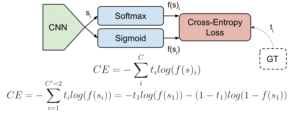","metadata":{}},{"cell_type":"code","source":"m = nn.LogSoftmax(dim=0)\n\ncriterion = nn.NLLLoss(reduction='none')\n\nx = torch.tensor(np.linspace(0,4,400).reshape(200,2), dtype=torch.float32) \ny = target[:200].long()#torch.ones(250, dtype=torch.long) # expect the target to be integer (Long)\n\nsparse_loss = criterion(m(x), y)","metadata":{"execution":{"iopub.status.busy":"2022-08-25T01:03:47.275021Z","iopub.execute_input":"2022-08-25T01:03:47.275477Z","iopub.status.idle":"2022-08-25T01:03:47.284981Z","shell.execute_reply.started":"2022-08-25T01:03:47.27544Z","shell.execute_reply":"2022-08-25T01:03:47.283878Z"},"trusted":true},"execution_count":null,"outputs":[]},{"cell_type":"code","source":"plt.style.use('seaborn')\nplt.figure(figsize=(8,6))\nplt.plot(x[:,0].numpy(), sparse_loss.softmax(dim=0).numpy(), 'r--', label='Sparse CE', linewidth=2.0 )\nplt.legend(loc=\"upper right\")\nplt.xlabel('$Y_{pred}$', fontsize=15)\nplt.ylabel(\"$L(y=1, f(x))$\", fontsize=15)\nplt.title('Loss Function', fontsize=15)\nplt.show()","metadata":{"execution":{"iopub.status.busy":"2022-08-25T01:05:23.689691Z","iopub.execute_input":"2022-08-25T01:05:23.69021Z","iopub.status.idle":"2022-08-25T01:05:23.971525Z","shell.execute_reply.started":"2022-08-25T01:05:23.690168Z","shell.execute_reply":"2022-08-25T01:05:23.970485Z"},"_kg_hide-input":true,"trusted":true},"execution_count":null,"outputs":[]},{"cell_type":"markdown","source":"# Kullback Leibler Divergence Loss\n---\n$$J(\\hat{y}, y) = y \\cdot \\log{\\frac{y}{\\hat{y}}} = y \\cdot (\\log{y} - \\log{\\hat{y}})$$\n\nTo avoid underflow issues when computing this quantity, this loss expects the argument input in the log-space. The argument target may also be provided in the log-space if `log_target= True`.","metadata":{}},{"cell_type":"code","source":"kl_loss = torch.nn.KLDivLoss(reduction='none', log_target=True) #specify whether the target is the log space\n# input should be a distribution in the log space\ninput_ = F.log_softmax(pred[:200], dim=0)\nlog_target = F.log_softmax(target[:200], dim=0)\noutput = kl_loss(input_, log_target)","metadata":{"execution":{"iopub.status.busy":"2022-08-25T01:04:41.666374Z","iopub.execute_input":"2022-08-25T01:04:41.666854Z","iopub.status.idle":"2022-08-25T01:04:41.674962Z","shell.execute_reply.started":"2022-08-25T01:04:41.666816Z","shell.execute_reply":"2022-08-25T01:04:41.673436Z"},"trusted":true},"execution_count":null,"outputs":[]},{"cell_type":"markdown","source":"# Visualization for Multi-Class Classification Loss Functions\n---","metadata":{}},{"cell_type":"code","source":"plt.style.use('seaborn')\nplt.figure(figsize=(8,6))\nplt.plot(pred[:200].numpy(), output.numpy(), 'orange', label='KLDiv Loss',linewidth=2.0 )\nplt.plot(pred[:200].numpy(), BCE_list_cat.softmax(dim=0).numpy(), 'b--', label='Softmax CE', linewidth=2.0 )\nplt.plot(x[:,0].numpy(), sparse_loss.softmax(dim=0).numpy(), 'r--', label='Sparse CE', linewidth=2.0 )\nplt.legend(loc=\"upper right\")\nplt.xlim(0,3)\nplt.xlabel('$Y_{pred}$', fontsize=15)\nplt.ylabel(\"$L(y=1, f(x))$\", fontsize=15)\nplt.title('Loss Functions', fontsize=15)\nplt.show()","metadata":{"execution":{"iopub.status.busy":"2022-08-25T01:04:57.015486Z","iopub.execute_input":"2022-08-25T01:04:57.01598Z","iopub.status.idle":"2022-08-25T01:04:57.292467Z","shell.execute_reply.started":"2022-08-25T01:04:57.015904Z","shell.execute_reply":"2022-08-25T01:04:57.291418Z"},"_kg_hide-input":true,"trusted":true},"execution_count":null,"outputs":[]},{"cell_type":"markdown","source":"\n\n
3. CONCLUSION⤒
\n\nTo sum up, I've walked through different loss functions, their usages, and how to select a suitable activation function for each classification task. The table below gives a snapshot of where to use each of these functions:\n\n","metadata":{}},{"cell_type":"markdown","source":"# References\n\n* [Visualizing Loss Functions](https://www.kaggle.com/code/mayank1101sharma/visualizing-loss-functions/notebook)\n* [Activation Functions and Loss Functions for Neural Networks-How to pick the right one?](https://medium.com/analytics-vidhya/activation-functions-and-loss-functions-for-neural-networks-how-to-pick-the-right-one-542e1dd523e0)\n* [Loss Function Library](https://www.kaggle.com/code/bigironsphere/loss-function-library-keras-pytorch/notebook)\n* [Guides to pytorch Loss Functions](https://neptune.ai/blog/pytorch-loss-functions)\n* [Loss functions comparison sklearn](https://scikit-learn.org/stable/auto_examples/linear_model/plot_sgd_loss_functions.html)\n","metadata":{}},{"cell_type":"markdown","source":"
If you find this notebook useful, do give me an upvote, it motivates me a lot.
This notebook is still a work in progress. Keep checking for further developments!😊
","metadata":{}},{"cell_type":"code","source":"","metadata":{},"execution_count":null,"outputs":[]}]}