{"metadata":{"kernelspec":{"language":"python","display_name":"Python 3","name":"python3"},"language_info":{"pygments_lexer":"ipython3","nbconvert_exporter":"python","version":"3.6.4","file_extension":".py","codemirror_mode":{"name":"ipython","version":3},"name":"python","mimetype":"text/x-python"}},"nbformat_minor":4,"nbformat":4,"cells":[{"cell_type":"code","source":"%%html\n","metadata":{"_uuid":"fc84fd93-736b-49ce-90c9-ae7597574959","_cell_guid":"60f6e4c2-02b4-4fc3-8c1a-3b1d408d2f7a","execution":{"iopub.status.busy":"2021-06-10T18:28:39.379318Z","iopub.execute_input":"2021-06-10T18:28:39.379647Z","iopub.status.idle":"2021-06-10T18:28:39.388827Z","shell.execute_reply.started":"2021-06-10T18:28:39.379614Z","shell.execute_reply":"2021-06-10T18:28:39.388095Z"},"trusted":true},"execution_count":null,"outputs":[]},{"cell_type":"markdown","source":"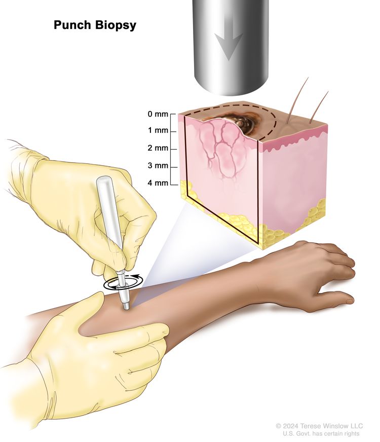","metadata":{}},{"cell_type":"markdown","source":"L'échelle de Clark comporte 5 niveaux de mélanome :\n\n 1. Les cellules se trouvent dans la couche externe de la peau (épiderme)\n\n 2. Les cellules se trouvent dans la couche située directement sous l'épiderme (derme pupillaire)\n\n 3. Les cellules touchent la couche suivante appelée derme profond\n\n 4. Les cellules se sont répandues dans le derme réticulaire\n\n 5. Les cellules se sont développées dans la couche de graisse\n\n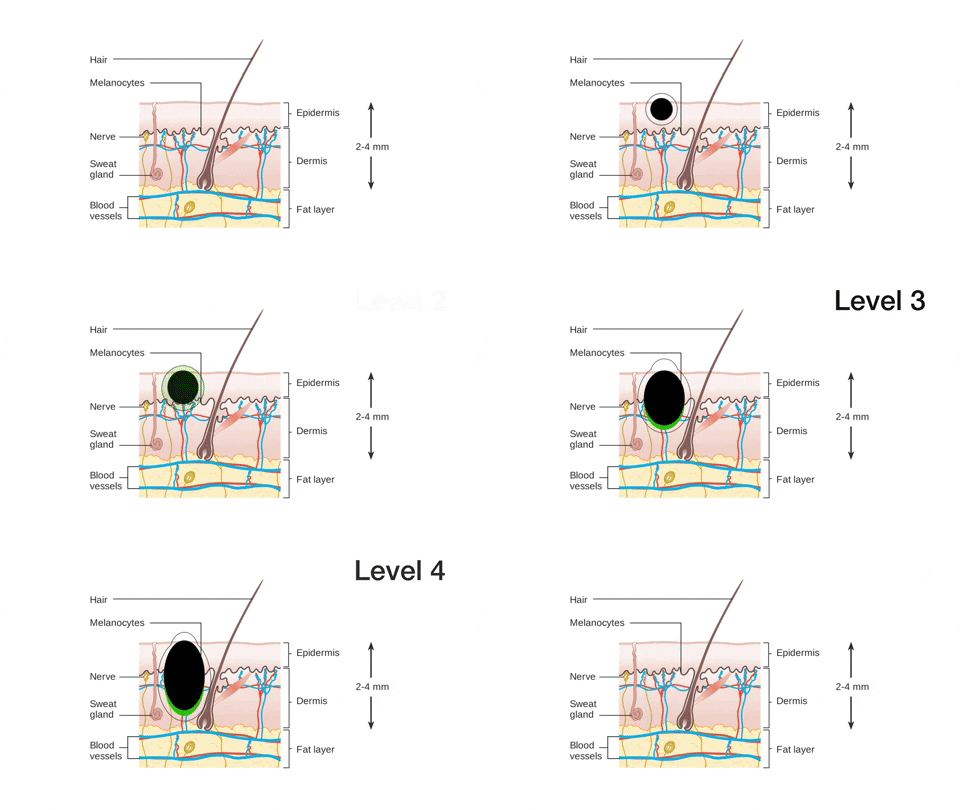","metadata":{}},{"cell_type":"markdown","source":"## Références \n* [TensorFlow + Transfer Learning: Melanoma](https://www.kaggle.com/amyjang/tensorflow-transfer-learning-melanoma)\n* [GENERAL INFORMATION ABOUT MELANOMA](https://www.uhhospitals.org/services/cancer-services/skin-cancer/melanoma/about-melanoma)\n","metadata":{}},{"cell_type":"markdown","source":"# 1. Introduction ▶\n\n### 1.1Qu'est-ce que le mélanome:\n* [Le mélanome est le cancer de la peau le moins fréquent mais le plus mortel, ne représentant qu'environ 1 % de tous les cas, mais la grande majorité des décès dus au cancer de la peau.](https://www.aimatmelanoma.org/about-melanoma/melanoma-stats-facts-and-figures/)\n* Le mélanome est le troisième cancer le plus fréquent chez les hommes et les femmes âgés de 20 à 39 ans.\n* Aux États-Unis, le mélanome continue d'être \n * le cinquième cancer le plus fréquent chez les hommes de tous les groupes d'âge\n * le sixième cancer le plus fréquent chez les femmes de tous les groupes d'âge\n* L'Australie et la Nouvelle-Zélande présentent la plus forte incidence de mélanomes au monde (plus de deux fois plus qu'en Amérique du Nord)\n\n\n# Nôtre Data:\n### Train Dataset se compose de:\n\n 1. image name -> le nom de fichier de l'image spécifique pour train set\n 2. patient_id -> id unique du patient \n 3. sex -> genre du patient\n 4. age_approx -> âge approximatif du patient \n 5. anatom_site_general_challenge -> l'emplacement du scan site\n 6. diagnosis -> des informations sur le diagnostic\n 7. benign_malignant - indique le résultat du scan s'il est malin ou bénin\n 8. target -> même chose que ci-dessus mais en mieux pour la modélisation puisqu'elle est binaire\n\n### Test Dataset se compose de:\n\n 1. image name -> le nom de fichier de l'image spécifique pour test set\n 2. patient_id -> id unique du patient \n 3. sex -> genre du patient\n 4. age_approx -> âge approximatif du patient \n 5. anatom_site_general_challenge -> l'emplacement du scan site\n\n\n\n\n### 1.2 objectifs:\n> L'objectif est d'identifier correctement les cas ****bénins**** et ****malins****. Une tumeur bénigne est une tumeur qui n'envahit pas les tissus environnants ou ne se propage pas dans le corps. Une tumeur maligne est une tumeur qui peut envahir les tissus environnants ou se propager dans le corps. .\n:max_bytes(150000):strip_icc():format(webp)/514240-article-img-malignant-vs-benign-tumor2111891f-54cc-47aa-8967-4cd5411fdb2f-5a2848f122fa3a0037c544be.png) \n\n> Data: DICOM Files split in Train (33,126 observations) and Test (10,982 observations)\n
\n\n> Data: DICOM Files split in Train (33,126 observations) and Test (10,982 observations)\n \n","metadata":{"_uuid":"5854a53e-93fc-421d-9b1d-17cf0a96942c","_cell_guid":"28b619f3-7bb6-42df-a1b7-6f74e0b38a35","trusted":true}},{"cell_type":"markdown","source":"# 3.Préparation de la base de données","metadata":{"_uuid":"10a84676-7471-469b-bfe2-82453e9a8142","_cell_guid":"7cea7dc2-21cd-4fb7-b9f8-dd56eaa53376","trusted":true}},{"cell_type":"markdown","source":"## Visualisation de données","metadata":{"_uuid":"2b058ab1-d122-4774-bca2-a70717e8ea6c","_cell_guid":"c6096c9f-29ed-43a4-a0ca-c79c71477e68","trusted":true}},{"cell_type":"code","source":"# Regular Imports\nimport os\nimport pandas as pd\nimport numpy as np\nimport seaborn as sns\nimport matplotlib.pyplot as plt\n%matplotlib inline\nimport matplotlib.image as mpimg\nfrom tabulate import tabulate\nimport missingno as msno \nfrom IPython.display import display_html\nfrom PIL import Image\nimport gc\nimport cv2\n\nimport pydicom # for DICOM images\nfrom skimage.transform import resize\n\n# SKLearn\nfrom sklearn.preprocessing import LabelEncoder\nfrom sklearn.preprocessing import OneHotEncoder\n\nimport warnings\nwarnings.filterwarnings(\"ignore\")\n\n\n# Set Style\nsns.set(style=\"darkgrid\")\nsns.despine(left=True, bottom=True)\n\n","metadata":{"_uuid":"d8e22e80-c430-419c-998c-e64565fa9422","_cell_guid":"34a5dd93-f673-45fd-bf29-cc5eb028a4ae","execution":{"iopub.status.busy":"2021-06-10T18:28:39.390296Z","iopub.execute_input":"2021-06-10T18:28:39.390755Z","iopub.status.idle":"2021-06-10T18:28:41.981204Z","shell.execute_reply.started":"2021-06-10T18:28:39.390714Z","shell.execute_reply":"2021-06-10T18:28:41.980247Z"},"trusted":true},"execution_count":null,"outputs":[]},{"cell_type":"code","source":"list(os.listdir('../input/siim-isic-melanoma-classification'))","metadata":{"execution":{"iopub.status.busy":"2021-06-10T18:28:41.98258Z","iopub.execute_input":"2021-06-10T18:28:41.982808Z","iopub.status.idle":"2021-06-10T18:28:41.989237Z","shell.execute_reply.started":"2021-06-10T18:28:41.982783Z","shell.execute_reply":"2021-06-10T18:28:41.988448Z"},"trusted":true},"execution_count":null,"outputs":[]},{"cell_type":"code","source":"# Directory\ndirectory = '../input/siim-isic-melanoma-classification'\n\n# Import the 2 csv s\ntrain_df = pd.read_csv(directory + '/train.csv')\ntest_df = pd.read_csv(directory + '/test.csv')\n\nprint('Train has {:,} rows and Test has {:,} rows.'.format(len(train_df), len(test_df)))\n\n# Change columns names\nnew_names = ['dcm_name', 'ID', 'sex', 'age', 'anatomy', 'diagnosis', 'benign_malignant', 'target']\ntrain_df.columns = new_names\ntest_df.columns = new_names[:5]","metadata":{"execution":{"iopub.status.busy":"2021-06-10T18:28:41.990511Z","iopub.execute_input":"2021-06-10T18:28:41.990755Z","iopub.status.idle":"2021-06-10T18:28:42.123691Z","shell.execute_reply.started":"2021-06-10T18:28:41.990729Z","shell.execute_reply":"2021-06-10T18:28:42.122647Z"},"trusted":true},"execution_count":null,"outputs":[]},{"cell_type":"code","source":"print(train_df)","metadata":{"_uuid":"eed03eb4-27e1-42aa-b9f6-5e7e93cf08f1","_cell_guid":"e61b4ef5-26b2-4b29-9bb1-6f604e214554","execution":{"iopub.status.busy":"2021-06-10T18:28:42.127404Z","iopub.execute_input":"2021-06-10T18:28:42.127772Z","iopub.status.idle":"2021-06-10T18:28:42.207746Z","shell.execute_reply.started":"2021-06-10T18:28:42.127731Z","shell.execute_reply":"2021-06-10T18:28:42.206902Z"},"trusted":true},"execution_count":null,"outputs":[]},{"cell_type":"code","source":"print(test_df)","metadata":{"_uuid":"7c39acbe-1eaa-4a6a-9af5-7a6ddcf144ea","_cell_guid":"9491ae4e-aa01-4411-8775-b87f3ddd3984","execution":{"iopub.status.busy":"2021-06-10T18:28:42.210893Z","iopub.execute_input":"2021-06-10T18:28:42.211145Z","iopub.status.idle":"2021-06-10T18:28:42.227438Z","shell.execute_reply.started":"2021-06-10T18:28:42.211117Z","shell.execute_reply":"2021-06-10T18:28:42.226507Z"},"trusted":true},"execution_count":null,"outputs":[]},{"cell_type":"code","source":"train_df.head()","metadata":{"_uuid":"dfbf294e-eede-41aa-bad8-3eeeb4f577a8","_cell_guid":"2cf4d1c1-134b-4b16-b366-a1b869c2224a","execution":{"iopub.status.busy":"2021-06-10T18:28:42.229362Z","iopub.execute_input":"2021-06-10T18:28:42.229733Z","iopub.status.idle":"2021-06-10T18:28:42.252796Z","shell.execute_reply.started":"2021-06-10T18:28:42.229692Z","shell.execute_reply":"2021-06-10T18:28:42.251819Z"},"trusted":true},"execution_count":null,"outputs":[]},{"cell_type":"code","source":"test_df.head()","metadata":{"_uuid":"31883da2-5cb8-42be-8837-6611ab72cb56","_cell_guid":"f27adfb7-514f-4a4a-9d3b-53d8a5ce837c","execution":{"iopub.status.busy":"2021-06-10T18:28:42.254231Z","iopub.execute_input":"2021-06-10T18:28:42.254764Z","iopub.status.idle":"2021-06-10T18:28:42.271757Z","shell.execute_reply.started":"2021-06-10T18:28:42.25472Z","shell.execute_reply":"2021-06-10T18:28:42.27061Z"},"trusted":true},"execution_count":null,"outputs":[]},{"cell_type":"code","source":"fig, (ax1, ax2) = plt.subplots(1, 2, figsize=(20,5))\nsns.countplot(ax=ax1, x=\"anatomy\", data=train_df)\nax1.set_title(\"distribution de anatomy dans training data\")\nsns.countplot(ax=ax2, x=\"anatomy\", data=test_df)\nax2.set_title(\"distribution de anatomy dans test data\")\nplt.show()","metadata":{"_uuid":"d347d94b-5cfb-46ec-af10-3f64bc8cc461","_cell_guid":"cc0e83d5-b6ac-4fb2-b367-cbefc19ef47a","execution":{"iopub.status.busy":"2021-06-10T18:28:42.273443Z","iopub.execute_input":"2021-06-10T18:28:42.273872Z","iopub.status.idle":"2021-06-10T18:28:42.732982Z","shell.execute_reply.started":"2021-06-10T18:28:42.273831Z","shell.execute_reply":"2021-06-10T18:28:42.732291Z"},"trusted":true},"execution_count":null,"outputs":[]},{"cell_type":"code","source":"plt.figure(figsize=(16, 6))\na = sns.countplot(data=train_df, x='benign_malignant', hue='anatomy')\n\nfor p in a.patches:\n a.annotate(format(p.get_height(), ','), \n (p.get_x() + p.get_width() / 2., \n p.get_height()), ha = 'center', va = 'center', \n xytext = (0, 4), textcoords = 'offset points')\n\nplt.title('distribution de Anatomy par Target', fontsize=16)\nsns.despine(left=True, bottom=True);","metadata":{"execution":{"iopub.status.busy":"2021-06-10T18:28:42.733984Z","iopub.execute_input":"2021-06-10T18:28:42.734304Z","iopub.status.idle":"2021-06-10T18:28:43.062208Z","shell.execute_reply.started":"2021-06-10T18:28:42.734278Z","shell.execute_reply":"2021-06-10T18:28:43.061516Z"},"trusted":true},"execution_count":null,"outputs":[]},{"cell_type":"markdown","source":"1. Il y a plus d'hommes que de femmes dans l'ensemble de données\n2. Cependant, les pourcentages sont presque les mêmes","metadata":{}},{"cell_type":"code","source":"f, (ax1, ax2) = plt.subplots(1, 2, figsize = (16, 6))\n\na = sns.countplot(train_df['anatomy'], ax=ax1)\nb = sns.countplot(train_df['diagnosis'], ax=ax2)\n\na.set_xticklabels(a.get_xticklabels(), rotation=35, ha=\"right\")\nb.set_xticklabels(b.get_xticklabels(), rotation=35, ha=\"right\")\n\nfor p in a.patches:\n a.annotate(format(p.get_height(), ','), \n (p.get_x() + p.get_width() / 2., \n p.get_height()), ha = 'center', va = 'center', \n xytext = (0, 4), textcoords = 'offset points')\n \nfor p in b.patches:\n b.annotate(format(p.get_height(), ','), \n (p.get_x() + p.get_width() / 2., \n p.get_height()), ha = 'center', va = 'center', \n xytext = (0, 4), textcoords = 'offset points')\n \nax1.set_title('Les fréquences de Anatomy', fontsize=16)\nax2.set_title('Les fréquences de Diagnosis', fontsize=16)\nsns.despine(left=True, bottom=True);","metadata":{"execution":{"iopub.status.busy":"2021-06-10T18:28:43.063496Z","iopub.execute_input":"2021-06-10T18:28:43.064006Z","iopub.status.idle":"2021-06-10T18:28:43.555388Z","shell.execute_reply.started":"2021-06-10T18:28:43.063975Z","shell.execute_reply":"2021-06-10T18:28:43.554608Z"},"trusted":true},"execution_count":null,"outputs":[]},{"cell_type":"code","source":"fig, (ax1) = plt.subplots(1,1, figsize=(20,5))\nsns.countplot(ax=ax1, x=\"benign_malignant\", data=train_df)\nax1.set_title(\"distribution de benign_malignant dans training data\")\nplt.show()","metadata":{"execution":{"iopub.status.busy":"2021-06-10T18:28:43.556442Z","iopub.execute_input":"2021-06-10T18:28:43.556816Z","iopub.status.idle":"2021-06-10T18:28:43.720152Z","shell.execute_reply.started":"2021-06-10T18:28:43.556789Z","shell.execute_reply":"2021-06-10T18:28:43.719429Z"},"trusted":true},"execution_count":null,"outputs":[]},{"cell_type":"code","source":"fig, (ax1, ax2) = plt.subplots(1, 2, figsize=(20,5))\nsns.countplot(ax=ax1, x=\"sex\", data=train_df)\nax1.set_title(\"distribution de sex dans training data\")\nsns.countplot(ax=ax2, x=\"sex\", data=test_df)\nax2.set_title(\"distribution de sex dans test data\")\nplt.show()","metadata":{"execution":{"iopub.status.busy":"2021-06-10T18:28:43.721196Z","iopub.execute_input":"2021-06-10T18:28:43.721579Z","iopub.status.idle":"2021-06-10T18:28:44.015758Z","shell.execute_reply.started":"2021-06-10T18:28:43.721549Z","shell.execute_reply":"2021-06-10T18:28:44.01509Z"},"trusted":true},"execution_count":null,"outputs":[]},{"cell_type":"code","source":"plt.figure(figsize=(16, 6))\na = sns.countplot(data=train_df, x='benign_malignant', hue='sex')\n\nfor p in a.patches:\n a.annotate(format(p.get_height(), ','), \n (p.get_x() + p.get_width() / 2., \n p.get_height()), ha = 'center', va = 'center', \n xytext = (0, 4), textcoords = 'offset points')\n\nplt.title('distribution de sex par target', fontsize=16)\nsns.despine(left=True, bottom=True);","metadata":{"execution":{"iopub.status.busy":"2021-06-10T18:28:44.016739Z","iopub.execute_input":"2021-06-10T18:28:44.017076Z","iopub.status.idle":"2021-06-10T18:28:44.247998Z","shell.execute_reply.started":"2021-06-10T18:28:44.017049Z","shell.execute_reply":"2021-06-10T18:28:44.246837Z"},"trusted":true},"execution_count":null,"outputs":[]},{"cell_type":"code","source":"fig, (ax1, ax2) = plt.subplots(1, 2, figsize=(20,5))\nsns.countplot(ax=ax1, x=\"age\", data=train_df)\nax1.set_title(\"distribution d'age dans training data\")\nsns.countplot(ax=ax2, x=\"age\", data=test_df)\nax2.set_title(\"distribution d'age dans test data\")\nplt.show()","metadata":{"execution":{"iopub.status.busy":"2021-06-10T18:28:44.249722Z","iopub.execute_input":"2021-06-10T18:28:44.250069Z","iopub.status.idle":"2021-06-10T18:28:44.96743Z","shell.execute_reply.started":"2021-06-10T18:28:44.250036Z","shell.execute_reply":"2021-06-10T18:28:44.966639Z"},"trusted":true},"execution_count":null,"outputs":[]},{"cell_type":"code","source":"fig, (ax1) = plt.subplots(1,1, figsize=(20,5))\nsns.countplot(ax=ax1, x=\"target\", data=train_df)\nax1.set_title(\"distribution d'age dans training data\")\nplt.show()","metadata":{"execution":{"iopub.status.busy":"2021-06-10T18:28:44.969031Z","iopub.execute_input":"2021-06-10T18:28:44.969294Z","iopub.status.idle":"2021-06-10T18:28:45.137743Z","shell.execute_reply.started":"2021-06-10T18:28:44.969266Z","shell.execute_reply":"2021-06-10T18:28:45.136836Z"},"trusted":true},"execution_count":null,"outputs":[]},{"cell_type":"markdown","source":"* **0=bénins**\n* **1=malins**","metadata":{}},{"cell_type":"code","source":"f, (ax1, ax2) = plt.subplots(1, 2, figsize = (16, 6))\n\na = sns.countplot(train_df[train_df['target']==0]['diagnosis'], ax=ax1)\nb = sns.countplot(train_df[train_df['target']==1]['diagnosis'], ax=ax2)\n\na.set_xticklabels(a.get_xticklabels(), rotation=35, ha=\"right\")\nb.set_xticklabels(b.get_xticklabels(), rotation=35, ha=\"right\")\n\nfor p in a.patches:\n a.annotate(format(p.get_height(), ','), \n (p.get_x() + p.get_width() / 2., \n p.get_height()), ha = 'center', va = 'center', \n xytext = (0, 4), textcoords = 'offset points')\n \nfor p in b.patches:\n b.annotate(format(p.get_height(), ','), \n (p.get_x() + p.get_width() / 2., \n p.get_height()), ha = 'center', va = 'center', \n xytext = (0, 4), textcoords = 'offset points')\n \nax1.set_title('Cas bénins: vue de diagnostic', fontsize=16)\nax2.set_title('Cas malins: vue de diagnostic', fontsize=16)\nsns.despine(left=True, bottom=True);","metadata":{"execution":{"iopub.status.busy":"2021-06-10T18:28:45.13953Z","iopub.execute_input":"2021-06-10T18:28:45.139883Z","iopub.status.idle":"2021-06-10T18:28:45.526775Z","shell.execute_reply.started":"2021-06-10T18:28:45.139839Z","shell.execute_reply":"2021-06-10T18:28:45.525778Z"},"trusted":true},"execution_count":null,"outputs":[]},{"cell_type":"code","source":"colors_nude = ['#e0798c','#65365a','#da8886','#cfc4c4','#dfd7ca']\npatients_count_train = train_df.groupby(by='ID')['dcm_name'].count().reset_index()\npatients_count_test = test_df.groupby(by='ID')['dcm_name'].count().reset_index()\n\n# Figure\nf, (ax1, ax2) = plt.subplots(1, 2, figsize = (16, 6))\n\na = sns.distplot(patients_count_train['dcm_name'], kde=False, bins=50, \n ax=ax1, color=colors_nude[0], hist_kws={'alpha': 1})\nb = sns.distplot(patients_count_test['dcm_name'], kde=False, bins=50, \n ax=ax2, color=colors_nude[1], hist_kws={'alpha': 1})\n \nax1.set_title('Train: Images per Patient Distribution', fontsize=16)\nax2.set_title('Test: Images per Patient Distribution', fontsize=16)\nsns.despine(left=True, bottom=True);\n","metadata":{"execution":{"iopub.status.busy":"2021-06-10T18:28:45.528141Z","iopub.execute_input":"2021-06-10T18:28:45.528381Z","iopub.status.idle":"2021-06-10T18:28:46.354174Z","shell.execute_reply.started":"2021-06-10T18:28:45.528353Z","shell.execute_reply":"2021-06-10T18:28:46.353163Z"},"trusted":true},"execution_count":null,"outputs":[]},{"cell_type":"code","source":"# Create the paths\npath_train = directory + '/train/' + train_df['dcm_name'] + '.dcm'\npath_test = directory + '/test/' + test_df['dcm_name'] + '.dcm'\n\n# Append to the original dataframes\ntrain_df['path_dicom'] = path_train\ntest_df['path_dicom'] = path_test\n\n# === JPEG ===\n# Create the paths\npath_train = directory + '/jpeg/train/' + train_df['dcm_name'] + '.jpg'\npath_test = directory + '/jpeg/test/' + test_df['dcm_name'] + '.jpg'\n\n# Append to the original dataframes\ntrain_df['path_jpeg'] = path_train\ntest_df['path_jpeg'] = path_test","metadata":{"execution":{"iopub.status.busy":"2021-06-10T18:28:46.355416Z","iopub.execute_input":"2021-06-10T18:28:46.355657Z","iopub.status.idle":"2021-06-10T18:28:46.544777Z","shell.execute_reply.started":"2021-06-10T18:28:46.35563Z","shell.execute_reply":"2021-06-10T18:28:46.544003Z"},"trusted":true},"execution_count":null,"outputs":[]},{"cell_type":"code","source":"fig, ax = plt.subplots()\nax.imshow(image)\nax.axis('off')","metadata":{},"execution_count":null,"outputs":[]},{"cell_type":"code","source":" plt.subplots(nrows=1, ncols=1, figsize=(16,6))","metadata":{},"execution_count":null,"outputs":[]},{"cell_type":"code","source":"data = pydicom.read_file(train_df['path_dicom'][0])\nimage = data.pixel_array\nfig, ax = plt.subplots(figsize=(16,16))\nimage = cv2.cvtColor(image, cv2.COLOR_RGB2GRAY)\nimage = cv2.resize(image, (512,512))\n#image=cv2.addWeighted(image, 4, cv2.GaussianBlur(image, (0,0) ,256/10), -4, 128)\nax.imshow(image, cmap=plt.cm.bone,) \nax.axis('off')","metadata":{"execution":{"iopub.status.busy":"2021-06-10T18:51:43.651387Z","iopub.execute_input":"2021-06-10T18:51:43.651731Z","iopub.status.idle":"2021-06-10T18:51:44.844016Z","shell.execute_reply.started":"2021-06-10T18:51:43.6517Z","shell.execute_reply":"2021-06-10T18:51:44.843054Z"},"trusted":true},"execution_count":null,"outputs":[]},{"cell_type":"code","source":"data = pydicom.read_file(train_df['path_dicom'][1])\nimage = data.pixel_array\nfig, ax = plt.subplots(figsize=(16,16))\n#image = cv2.cvtColor(image)\nimage = cv2.resize(image, (512,512))\n#image=cv2.addWeighted(image, 4, cv2.GaussianBlur(image, (0,0) ,256/10), -4, 128)\nax.imshow(image, cmap=plt.cm.bone,) \nax.axis('off')","metadata":{"execution":{"iopub.status.busy":"2021-06-10T18:57:35.612854Z","iopub.execute_input":"2021-06-10T18:57:35.613162Z","iopub.status.idle":"2021-06-10T18:57:36.929639Z","shell.execute_reply.started":"2021-06-10T18:57:35.613133Z","shell.execute_reply":"2021-06-10T18:57:36.920056Z"},"trusted":true},"execution_count":null,"outputs":[]},{"cell_type":"code","source":"data = pydicom.read_file(train_df['path_dicom'][2])\nimage = data.pixel_array\nfig, ax = plt.subplots(figsize=(16,16))\nimage = cv2.cvtColor(image, cv2.COLOR_RGB2GRAY)\nimage = cv2.resize(image, (512,512))\nax.imshow(image, cmap=plt.cm.bone,) \nax.axis('off')","metadata":{"execution":{"iopub.status.busy":"2021-06-10T18:52:07.740462Z","iopub.execute_input":"2021-06-10T18:52:07.740782Z","iopub.status.idle":"2021-06-10T18:52:08.502613Z","shell.execute_reply.started":"2021-06-10T18:52:07.740752Z","shell.execute_reply":"2021-06-10T18:52:08.501571Z"},"trusted":true},"execution_count":null,"outputs":[]},{"cell_type":"code","source":"data = pydicom.read_file(train_df['path_dicom'][3])\nimage = data.pixel_array\nfig, ax = plt.subplots(figsize=(16,16))\nimage = cv2.cvtColor(image, cv2.COLOR_RGB2GRAY)\nimage = cv2.resize(image, (512,512))\n#image=cv2.addWeighted(image, 4, cv2.GaussianBlur(image, (0,0) ,256/10), -4, 128)\nax.imshow(image, cmap=plt.cm.bone,) \nax.axis('off')","metadata":{"execution":{"iopub.status.busy":"2021-06-10T18:45:41.212842Z","iopub.execute_input":"2021-06-10T18:45:41.213317Z","iopub.status.idle":"2021-06-10T18:45:42.735705Z","shell.execute_reply.started":"2021-06-10T18:45:41.213272Z","shell.execute_reply":"2021-06-10T18:45:42.734631Z"},"trusted":true},"execution_count":null,"outputs":[]},{"cell_type":"code","source":"data = pydicom.read_file(train_df['path_dicom'][4])\nimage = data.pixel_array\nfig, ax = plt.subplots(figsize=(16,16))\nimage = cv2.cvtColor(image, cv2.COLOR_RGB2GRAY)\nimage = cv2.resize(image, (512,512))\n#image=cv2.addWeighted(image, 4, cv2.GaussianBlur(image, (0,0) ,256/10), -4, 128)\nax.imshow(image, cmap=plt.cm.bone,) \nax.axis('off')","metadata":{},"execution_count":null,"outputs":[]},{"cell_type":"code","source":"data = pydicom.read_file(train_df['path_dicom'][5])\nimage = data.pixel_array\nfig, ax = plt.subplots(figsize=(16,16))\nimage = cv2.cvtColor(image, cv2.COLOR_RGB2GRAY)\nimage = cv2.resize(image, (512,512))\n#image=cv2.addWeighted(image, 4, cv2.GaussianBlur(image, (0,0) ,256/10), -4, 128)\nax.imshow(image, cmap=plt.cm.bone,) \nax.axis('off')","metadata":{},"execution_count":null,"outputs":[]},{"cell_type":"code","source":"","metadata":{},"execution_count":null,"outputs":[]},{"cell_type":"code","source":"","metadata":{},"execution_count":null,"outputs":[]},{"cell_type":"code","source":"","metadata":{},"execution_count":null,"outputs":[]},{"cell_type":"code","source":"","metadata":{},"execution_count":null,"outputs":[]},{"cell_type":"code","source":"","metadata":{},"execution_count":null,"outputs":[]},{"cell_type":"code","source":"def show_images(data, n = 5, rows=1, cols=6, title='Default'):\n plt.figure(figsize=(16,4))\n\n for k, path in enumerate(data['path_dicom'][:n]):\n image = pydicom.read_file(path)\n image = image.pixel_array\n \n # image = resize(image, (200, 200), anti_aliasing=True)\n\n plt.suptitle(title, fontsize = 16)\n plt.subplot(rows, cols, k+1)\n plt.imshow(image)\n plt.axis('off')","metadata":{"execution":{"iopub.status.busy":"2021-06-10T18:28:46.545778Z","iopub.execute_input":"2021-06-10T18:28:46.546126Z","iopub.status.idle":"2021-06-10T18:28:46.553105Z","shell.execute_reply.started":"2021-06-10T18:28:46.5461Z","shell.execute_reply":"2021-06-10T18:28:46.552326Z"},"trusted":true},"execution_count":null,"outputs":[]},{"cell_type":"code","source":"show_images(train_df[train_df['target'] == 0], n=10, rows=2, cols=5, title='Benign Sample')","metadata":{"execution":{"iopub.status.busy":"2021-06-10T18:28:46.554187Z","iopub.execute_input":"2021-06-10T18:28:46.554538Z","iopub.status.idle":"2021-06-10T18:29:02.050737Z","shell.execute_reply.started":"2021-06-10T18:28:46.554504Z","shell.execute_reply":"2021-06-10T18:29:02.049825Z"},"trusted":true},"execution_count":null,"outputs":[]},{"cell_type":"code","source":"fig, axes = plt.subplots(nrows=1, ncols=1, figsize=(16,6))\nplt.suptitle(\"B&W\", fontsize = 16)\n\nfor i in range(0, 1):\n data = pydicom.read_file(train_df['path_dicom'][i])\n image = data.pixel_array\n \n # Transform to B&W\n # The function converts an input image from one color space to another.\n image = cv2.cvtColor(image, cv2.COLOR_RGB2GRAY)\n image = cv2.resize(image, (200,200))\n \n x = i \n y = i \n axes[x, y].imshow(image, cmap=plt.cm.bone) \n axes[x, y].axis('off')","metadata":{"execution":{"iopub.status.busy":"2021-06-10T18:38:56.52003Z","iopub.execute_input":"2021-06-10T18:38:56.520392Z","iopub.status.idle":"2021-06-10T18:38:57.466484Z","shell.execute_reply.started":"2021-06-10T18:38:56.520359Z","shell.execute_reply":"2021-06-10T18:38:57.465195Z"},"trusted":true},"execution_count":null,"outputs":[]},{"cell_type":"code","source":"fig, axes = plt.subplots(nrows=1, ncols=6, figsize=(16,6))\nplt.suptitle(\"Without Gaussian Blur\", fontsize = 16)\n\nfor i in range(0, 2*6):\n data = pydicom.read_file(train_df['path_dicom'][i])\n image = data.pixel_array\n \n # Transform to B&W\n # The function converts an input image from one color space to another.\n image = cv2.cvtColor(image, cv2.COLOR_RGB2HSV)\n image = cv2.resize(image, (200,200))\n \n x = i // 6\n y = i % 6\n axes[x, y].imshow(image, cmap=plt.cm.bone) \n axes[x, y].axis('off')","metadata":{"execution":{"iopub.status.busy":"2021-06-10T18:29:04.02906Z","iopub.status.idle":"2021-06-10T18:29:04.029497Z"},"trusted":true},"execution_count":null,"outputs":[]},{"cell_type":"code","source":"fig, axes = plt.subplots(nrows=1, ncols=6, figsize=(16,6))\nplt.suptitle(\"With Gaussian Blur\", fontsize = 16)\n\nfor i in range(0, 2*6):\n data = pydicom.read_file(train_df['path_dicom'][i])\n image = data.pixel_array\n \n # Transform to B&W\n # The function converts an input image from one color space to another.\n image = cv2.cvtColor(image, cv2.COLOR_RGB2HSV)\n image = cv2.resize(image, (200,200))\n image=cv2.addWeighted(image, 4, cv2.GaussianBlur(image, (0,0) ,256/10), -4, 128)\n \n x = i // 6\n y = i % 6\n axes[x, y].imshow(image, cmap=plt.cm.bone) \n axes[x, y].axis('off')","metadata":{"execution":{"iopub.status.busy":"2021-06-10T18:29:04.030324Z","iopub.status.idle":"2021-06-10T18:29:04.03074Z"},"trusted":true},"execution_count":null,"outputs":[]},{"cell_type":"code","source":"fig, axes = plt.subplots(nrows=1, ncols=6, figsize=(16,6))\nplt.suptitle(\"Hue, Saturation, Brightness\", fontsize = 16)\n\nfor i in range(0, 2*6):\n data = pydicom.read_file(train_df['path_dicom'][i])\n image = data.pixel_array\n \n # Transform to B&W\n # The function converts an input image from one color space to another.\n image = cv2.cvtColor(image, cv2.COLOR_RGB2HLS)\n image = cv2.resize(image, (200,200))\n \n x = i // 6\n y = i % 6\n axes[x, y].imshow(image, cmap=plt.cm.bone) \n axes[x, y].axis('off')","metadata":{"execution":{"iopub.status.busy":"2021-06-10T18:29:04.031543Z","iopub.status.idle":"2021-06-10T18:29:04.03215Z"},"trusted":true},"execution_count":null,"outputs":[]},{"cell_type":"code","source":"fig, axes = plt.subplots(nrows=1, ncols=6, figsize=(16,6))\nplt.suptitle(\"LUV Color Space\", fontsize = 16)\n\nfor i in range(0, 2*6):\n data = pydicom.read_file(train_df['path_dicom'][i])\n image = data.pixel_array\n \n # Transform to B&W\n # The function converts an input image from one color space to another.\n image = cv2.cvtColor(image, cv2.COLOR_RGB2LUV)\n image = cv2.resize(image, (200,200))\n \n x = i // 6\n y = i % 6\n axes[x, y].imshow(image, cmap=plt.cm.bone) \n axes[x, y].axis('off')\n\n","metadata":{"execution":{"iopub.status.busy":"2021-06-10T18:29:04.033545Z","iopub.status.idle":"2021-06-10T18:29:04.034262Z"},"trusted":true},"execution_count":null,"outputs":[]},{"cell_type":"code","source":"image_list","metadata":{"execution":{"iopub.status.busy":"2021-06-10T18:59:31.543873Z","iopub.execute_input":"2021-06-10T18:59:31.544361Z","iopub.status.idle":"2021-06-10T18:59:31.549795Z","shell.execute_reply.started":"2021-06-10T18:59:31.544327Z","shell.execute_reply":"2021-06-10T18:59:31.548885Z"},"trusted":true},"execution_count":null,"outputs":[]},{"cell_type":"code","source":"train_df","metadata":{"execution":{"iopub.status.busy":"2021-06-10T19:01:59.017331Z","iopub.execute_input":"2021-06-10T19:01:59.017654Z","iopub.status.idle":"2021-06-10T19:01:59.045207Z","shell.execute_reply.started":"2021-06-10T19:01:59.017622Z","shell.execute_reply":"2021-06-10T19:01:59.044315Z"},"trusted":true},"execution_count":null,"outputs":[]},{"cell_type":"code","source":"t0=train_df['path_jpeg'][0]\nt1=train_df['path_jpeg'][1]\nt2=train_df['path_jpeg'][2]\nt3=train_df['path_jpeg'][3]\nt4=train_df['path_jpeg'][4]\nt5=train_df['path_jpeg'][5]","metadata":{"execution":{"iopub.status.busy":"2021-06-10T19:02:18.695692Z","iopub.execute_input":"2021-06-10T19:02:18.696405Z","iopub.status.idle":"2021-06-10T19:02:18.701817Z","shell.execute_reply.started":"2021-06-10T19:02:18.696356Z","shell.execute_reply":"2021-06-10T19:02:18.700758Z"},"trusted":true},"execution_count":null,"outputs":[]},{"cell_type":"code","source":"#image_list = train_df.sample(20)['path_jpeg']\n#image_list = image_list.reset_index()['path_jpeg']\n\n# Show the sample\nplt.figure(figsize=(16,16))\n#plt.suptitle(\"Original View\", fontsize = 16)\n \n\nimage = mpimg.imread(t0)\nimage = cv2.resize(image, (512,512))\n#plt.subplot(2, 6, k+1)\nplt.imshow(image)\nplt.axis('off')","metadata":{},"execution_count":null,"outputs":[]},{"cell_type":"code","source":"#image_list = train_df.sample(20)['path_jpeg']\n#image_list = image_list.reset_index()['path_jpeg']\n\n# Show the sample\nplt.figure(figsize=(16,16))\n#plt.suptitle(\"Original View\", fontsize = 16)\n \n\nimage = mpimg.imread(t1)\nimage = cv2.resize(image, (512,512))\n#plt.subplot(2, 6, k+1)\nplt.imshow(image)\nplt.axis('off')","metadata":{},"execution_count":null,"outputs":[]},{"cell_type":"code","source":"#image_list = train_df.sample(20)['path_jpeg']\n#image_list = image_list.reset_index()['path_jpeg']\n\n# Show the sample\nplt.figure(figsize=(16,16))\n#plt.suptitle(\"Original View\", fontsize = 16)\n \n\nimage = mpimg.imread(t2)\nimage = cv2.resize(image, (512,512))\n#plt.subplot(2, 6, k+1)\nplt.imshow(image)\nplt.axis('off')","metadata":{},"execution_count":null,"outputs":[]},{"cell_type":"code","source":"#image_list = train_df.sample(20)['path_jpeg']\n#image_list = image_list.reset_index()['path_jpeg']\n\n# Show the sample\nplt.figure(figsize=(16,16))\n#plt.suptitle(\"Original View\", fontsize = 16)\n \n\nimage = mpimg.imread(t3)\nimage = cv2.resize(image, (512,512))\n#plt.subplot(2, 6, k+1)\nplt.imshow(image)\nplt.axis('off')","metadata":{},"execution_count":null,"outputs":[]},{"cell_type":"code","source":"#image_list = train_df.sample(20)['path_jpeg']\n#image_list = image_list.reset_index()['path_jpeg']\n\n# Show the sample\nplt.figure(figsize=(16,16))\n#plt.suptitle(\"Original View\", fontsize = 16)\n \n\nimage = mpimg.imread(t4)\nimage = cv2.resize(image, (512,512))\n#plt.subplot(2, 6, k+1)\nplt.imshow(image)\nplt.axis('off')","metadata":{},"execution_count":null,"outputs":[]},{"cell_type":"code","source":"#image_list = train_df.sample(20)['path_jpeg']\n#image_list = image_list.reset_index()['path_jpeg']\n\n# Show the sample\nplt.figure(figsize=(16,16))\n#plt.suptitle(\"Original View\", fontsize = 16)\n \n\nimage = mpimg.imread(t5)\nimage = cv2.resize(image, (512,512))\n#plt.subplot(2, 6, k+1)\nplt.imshow(image)\nplt.axis('off')","metadata":{},"execution_count":null,"outputs":[]},{"cell_type":"code","source":"#image_list = train_df.sample(20)['path_jpeg']\n#image_list = image_list.reset_index()['path_jpeg']\n\n# Show the sample\nplt.figure(figsize=(16,16))\n#plt.suptitle(\"Original View\", fontsize = 16)\n \n\nimage = mpimg.imread(t6)\nimage = cv2.resize(image, (512,512))\n#plt.subplot(2, 6, k+1)\nplt.imshow(image)\nplt.axis('off')","metadata":{},"execution_count":null,"outputs":[]},{"cell_type":"code","source":"","metadata":{},"execution_count":null,"outputs":[]},{"cell_type":"code","source":"","metadata":{},"execution_count":null,"outputs":[]},{"cell_type":"code","source":"","metadata":{},"execution_count":null,"outputs":[]},{"cell_type":"code","source":"","metadata":{},"execution_count":null,"outputs":[]},{"cell_type":"code","source":"#image_list = train_df.sample(20)['path_jpeg']\n#image_list = image_list.reset_index()['path_jpeg']\n\n# Show the sample\nplt.figure(figsize=(16,16))\n#plt.suptitle(\"Original View\", fontsize = 16)\n \n\nimage = mpimg.imread(t0)\nimage = cv2.resize(image, (512,512))\n#plt.subplot(2, 6, k+1)\nplt.imshow(image)\nplt.axis('off')\n","metadata":{"execution":{"iopub.status.busy":"2021-06-10T19:02:50.665379Z","iopub.execute_input":"2021-06-10T19:02:50.665695Z","iopub.status.idle":"2021-06-10T19:02:51.925298Z","shell.execute_reply.started":"2021-06-10T19:02:50.665667Z","shell.execute_reply":"2021-06-10T19:02:51.924284Z"},"trusted":true},"execution_count":null,"outputs":[]}]}