
First, we thank the competition hosts @evancalabrese, @shosys and every person involved from RSNA in data preparation and competition related process, and Kaggle staff for organizing this competition.
\nBelow, we introduce the solution of team Vibes and Genius Trade-Off -- @tom99763, @sersasj, @iamparadox, @chihantsai, @atom1231!
\nTL;DR
\nOur solution combines three complementary approaches:
\nThe final probabilities are obtained by averaging the outputs of the YOLO 2.5D models, 3D CenterNet with 2D Effv2s extractor and the three meta-classifiers.
\nHere is the diagram of our approach.
\nWe used two different variations of YOLO:
\ntimm/tf_efficientnetv2_s.in21k_ft_in1k as the backboneFor details about the YOLO+timm customization, please refer to the BYU writeup.
\nWe treated each of the 13 vessel locations as separate bounding box classes:
\nImages were resized to 512×512, normalized with min-max and converted to 2.5D variation:
\nR (Red channel) = slice i-1\nG (Green channel) = slice i\nB (Blue channel) = slice i+1
The figure below shows examples of slices in 2D vs 2.5D variation:
\n
As can be seen in the examples, the images vary significantly because we didn't standardize Z spacing.
\nI (@sersasj) spent 1-2 weeks experimenting with Z-axis resize, but results were consistently worse. Perhaps I was doing something wrong, but didn't have time to investigate further.
\nWe were very reluctant to try 2.5D without proper Z-spacing resize (in my mind didn’t seem a good idea - @sersasj). Nevertheless, the 2.5D approach even without Z-resampling improved results by 0.02+ in CV.
\nData Sampling Strategy:
\nFor negative samples we took 10 evenly sampled slices per series.
\nExample: For a 100-slice series → slices [1, 11, 22, 33, 44, 56, 67, 78, 89, 99]
\nFor positive samples we used all slices containing annotations
\n \n \n \n \n \n \n \n \n \n \n \n \n \n \n \n \n \n \nWe also modified the fitness function to include auc metric and prioritize mAP@50.
\nfitness = × mAP@ + × mAP@- + × mAUC\nDid this help? Maybe a little. In the BYU competition, we had already found that prioritizing mAP@50 over the Ultralytics standard 1.0×mAP@50-95 gave better results.
\nAdding AUC seemed like a good idea at the time since it's the competition metric, but we didn't investigate thoroughly whether it significantly improved performance. It's possible the benefit was marginal, but we kept it for consistency.
\nTraining Hardware and Time
\n| Hardware Setup | \nGPU | \nCPU | \nRAM | \nTime per Fold | \nTotal (5 folds) | \n
|---|---|---|---|---|---|
| @sersasj | \nRTX 3090 | \nIntel Core i5-12400F (12) @ 4.4GHz | \n32GB | \n4-5 hours | \n~24 hours | \n
| @iamparadox | \nRTX 4090 | \nAMD Ryzen 9 7950X (32) @ 5.883GHz | \n64GB | \n~2 hours | \n~10 hours | \n
For inference, we sort DICOM slices by spatial position (SliceLocation → ImagePositionPatient → InstanceNumber), create 2.5D triplets for slices 1 to N-1
\nRun batch inference across both models, extract max confidence per class and use max(localization_confidences) as overall aneurysm presence probability
\nThe process can be observed in the gif below:
\n.gif?generation=1761065820372307&alt=media\")
folds were stratified using MultilabelStratifiedKFold to ensure balanced distribution across:
| Fold | \nloc_macro_auc | \ncls_auc | \ncombined_mean | \n
|---|---|---|---|
| fold0 | \n0.8184 | \n0.7549 | \n0.7867 | \n
| fold1 | \n0.8114 | \n0.7897 | \n0.8005 | \n
| fold2 | \n0.8134 | \n0.7827 | \n0.7981 | \n
| fold3 | \n0.8162 | \n0.7872 | \n0.8017 | \n
| fold4 | \n0.8540 | \n0.8281 | \n0.8410 | \n
| Average | \n0.8227 | \n0.7885 | \n0.8056 | \n
| Fold | \nloc_macro_auc | \ncls_auc | \ncombined_mean | \n
|---|---|---|---|
| fold0 | \n0.7978 | \n0.7790 | \n0.7884 | \n
| fold1 | \n0.8159 | \n0.8269 | \n0.8214 | \n
| fold2 | \n0.8155 | \n0.7921 | \n0.8038 | \n
| fold3 | \n0.8153 | \n0.7907 | \n0.8030 | \n
| fold4 | \n0.8499 | \n0.8560 | \n0.8529 | \n
| Average | \n0.8189 | \n0.8090 | \n0.8139 | \n
| Fold | \nloc_macro_auc | \ncls_auc | \ncombined_mean | \n
|---|---|---|---|
| fold0 | \n0.8393 | \n0.7849 | \n0.8121 | \n
| fold1 | \n0.8330 | \n0.8291 | \n0.8310 | \n
| fold2 | \n0.8399 | \n0.8135 | \n0.8267 | \n
| fold3 | \n0.8370 | \n0.8093 | \n0.8232 | \n
| fold4 | \n0.8738 | \n0.8620 | \n0.8679 | \n
| Average | \n0.8446 | \n0.8198 | \n0.8322 | \n
In the initial stages of YOLO development @sersasj created an ensemble with 3xYolo11m and 0.69LB EfficientNetB2 public notebook. That gave us a score of 0.78 LB and put us in the top 3 in early stages of competition
\nAfter a bit of probing the leaderboard, @iamparadox found out that YOLO's aneurysm classification AUROC was very low (around ~0.58). Then we started to develop models that would complement YOLO and boost the aneurysm classification AUROC. (We later discovered that the poor results of early YOLO development were due to an insufficient amount of negative samples in training.)
\nOne of the class of models that we used was 2.5D models that just detects the presence of aneurysm in the given series with auxiliary segmentation head. These models were inspired by https://www.kaggle.com/code/hengck23/3d-unet-using-2d-image-encoder. These models in combination with yolo11m gave us a LB of 0.80.
\nThese models then became obsolete when we merged with @chihantsai, @atom1231.
\nIn the BYU competition, our best-performing backbone was timm/convnextv2_base.fcmae_ft_in22k_in1k. However, in the current competition, training with half precision caused the loss to quickly become NaN. Based on our investigation, this appears to be a common issue with ConvNeXt architectures. We hypothesize that if trained in full precision, this backbone could achieve performance comparable to YOLO11m and timm/tf_efficientnetv2_s.in21k_ft_in1k. Unfortunately, we were unable to verify this due to time constraints.
Modifying the neck and head was also considered. From what we investigate with @tatamikenn awesome reverse engineer notebook P3 features appeared to be the most utilized. We conducted a quick test on a single fold, but results on validation were more or less the same so we decided to move on.
\n.png?generation=1760534911466456&alt=media\")
We also try to use our 3d segmentation result to filter out invalid location prediction from yolo, but recall drops a lot.
\nMoreover, we tried extracting patches using YOLO and applying wavelet and log-polar transforms to the patches before predicting their classes; however, this approach did not yield good results.
This is a highly experimental project, made with a lot of help from AI. We started with the popular “LB 0.69 Public Notebook” , reconstructed the entire training pipeline and data preprocessing from it, and then incorporated a CenterNet-like mechanism to detect the center of the aneurysms.
\nWe adopt a slice-wise 2D encoder + shallow 3D head design:
\ntf_efficientnetv2_s.in21k_ft_in1k) from timm in features_only mode with the penultimate feature map (out_indices = (1,-2)).(B, C=1, D, H, W) is rearranged into B·D 2D slices, encoded independently, then reassembled to (B, C_feat, D, H′, W′) before the 3D head. If the backbone expects 3 channels, single-channel inputs are channel-repeated.base_channels) aggregates signals across depth.num_classes = 13 vessel locations (3D centerness maps)(dz, dy, dx)(D, H, W); map to the output grid using (stride_d=1, stride_h=stride_w=16) so the output is D × H/16 × W/16.Vessel masks are produced in physical space by training a 3D DynUNet on volumes resampled to 0.7 mm isotropic spacing. The provided voxel-level annotations of 13 vessel classes are merged into a single binary vessel mask for training. The resulting 3D masks are then converted to slice-wise 2D masks to supervise the auxiliary head.
\nWe train with four terms and sum them with weights:
\nGiven heatmap logits H ∈ ℝ^{B×13×D×H′×W′}:
Per-class series logits: spatial max over (D, H′, W′) for each of the 13 classes.
Aneurysm Present (global) logit: the max over the 13 class logits.
\nThese 14 logits drive the BCE loss and are exported for meta-ensembling.
.npy volumes; (D,H,W) expanded to (1,D,H,W)— here D = 64.T_max = epochs, eta_min = 1e-6); StepLR / ReduceLROnPlateau also supported.1, lateral 16pretrained=True, not frozen by default| Fold | \nloc_macro_auc | \ncls_auc | \ncombined_mean | \n
|---|---|---|---|
| fold0 | \n0.7762 | \n0.7747 | \n0.7754 | \n
| fold1 | \n0.7676 | \n0.8069 | \n0.7873 | \n
| fold2 | \n0.7508 | \n0.7892 | \n0.7700 | \n
| fold3 | \n0.7553 | \n0.7778 | \n0.7666 | \n
| fold4 | \n0.7734 | \n0.7758 | \n0.7746 | \n
| Average | \n0.7647 | \n0.7848 | \n0.7748 | \n
| Fold | \nloc_macro_auc | \ncls_auc | \ncombined_mean | \n
|---|---|---|---|
| fold0 | \n0.7779 | \n0.7991 | \n0.7885 | \n
| fold1 | \n0.7828 | \n0.7987 | \n0.7908 | \n
| fold2 | \n0.7601 | \n0.8051 | \n0.7826 | \n
| fold3 | \n0.7683 | \n0.7826 | \n0.7755 | \n
| fold4 | \n0.7586 | \n0.7954 | \n0.7770 | \n
| Average | \n0.7695 | \n0.7962 | \n0.7829 | \n
Flayer converts 2D EfficientNetV2-S slice features into 3D evidence maps with a light 3D head, supervises them using CenterNet-style heatmaps + offsets, and produces robust 14-logit series-level predictions (including an aggregated aneurysm present logit) that plug cleanly into our stacked meta-classifier.
\nWe designed a stacked ensemble architecture to integrate predictions from YOLO11m, YOLO11-EffV2s, and EffV2s-3D-CenterNet models. Specifically, each meta-classifier receives the concatenated predictions from all base models as input and produces final predictions for both aneurysm presence and location-specific detection. This setup enables the model to assess the presence of an aneurysm at a given location by considering predictions from all locations across all models, effectively capturing the ensemble’s collective reasoning about aneurysm presence.
\n\nmetadata = np.array([age, sex])\nX = np.concatenate([np.array([yolo11m_cls_preds[fold_id]]), yolo11m_loc_preds[fold_id],\n np.array([effv2s_cls_preds[fold_id]]), effv2s_loc_preds[fold_id],\n flayer_fold_preds[fold_id], metadata], axis=)[, :]\nlgb_pred = predict_prob_lgb(X, fold_id) \nxgb_pred = predict_prob_xgb(X, fold_id)\ncat_pred = predict_prob_cat(X, fold_id)\nWe experimented with two ensemble structures:
\n( features, [() + flayer() + meta()])\n( features, [yolo11m() + ()+ () + ()])\n
\nThis comparison allows us to evaluate whether combining multiple feature streams in parallel provides additional complementary information beyond the sequential (series) configuration.
We found that combining predictions from different YOLO backbones and flayer in parallel provides better improvement than series in the ensemble CV score. This suggests that the GBDT effectively leverages each model’s perception of aneurysm presence across locations to make accurate judgments. We were unable to complete the 5-fold submission due to issues encountered on the final day. Therefore, we present here our final selected result, which is based on the average of 2 folds.
\n| \n | Series | \nParallel | \n
|---|---|---|
| 5 folds CV (average) | \n0.84 | \n0.852 | \n
| 5 folds CV (nelder-mead optimized) | \n0.841 | \n0.858 | \n
| public score (average; 2 folds) | \n0.83 | \n0.83082 | \n
| private score (average; 2 folds) | \n0.81 | \n0.8230 | \n
We’ve also tried Keypoint-Based Dual-Graph Predictor in Tom’s BYU approach earlier and found it performed well in terms of ensemble CV performance. However, the YOLO-based feature extraction and preprocessing were too time-consuming and often led to timeouts. Therefore, we did not include this method in our final solution.
\nSubmission:
\n\nMeta classifier training: 2x yolo + flayer meta training (final ver)
\nGithub: 9th-place-solution-yolo-RSNA-IAD
", "messages": [ { "id": 3302294, "postDate": "2025-10-15T13:34:16.853Z", "content": "First, we thank the competition hosts @evancalabrese, @shosys and every person involved from RSNA in data preparation and competition related process, and Kaggle staff for organizing this competition.
\nBelow, we introduce the solution of team Vibes and Genius Trade-Off -- @tom99763, @sersasj, @iamparadox, @chihantsai, @atom1231!
\nTL;DR
\nOur solution combines three complementary approaches:
\nThe final probabilities are obtained by averaging the outputs of the YOLO 2.5D models, 3D CenterNet with 2D Effv2s extractor and the three meta-classifiers.
\nHere is the diagram of our approach.
\nWe used two different variations of YOLO:
\ntimm/tf_efficientnetv2_s.in21k_ft_in1k as the backboneFor details about the YOLO+timm customization, please refer to the BYU writeup.
\nWe treated each of the 13 vessel locations as separate bounding box classes:
\nImages were resized to 512×512, normalized with min-max and converted to 2.5D variation:
\nR (Red channel) = slice i-1\nG (Green channel) = slice i\nB (Blue channel) = slice i+1
The figure below shows examples of slices in 2D vs 2.5D variation:
\n
As can be seen in the examples, the images vary significantly because we didn't standardize Z spacing.
\nI (@sersasj) spent 1-2 weeks experimenting with Z-axis resize, but results were consistently worse. Perhaps I was doing something wrong, but didn't have time to investigate further.
\nWe were very reluctant to try 2.5D without proper Z-spacing resize (in my mind didn’t seem a good idea - @sersasj). Nevertheless, the 2.5D approach even without Z-resampling improved results by 0.02+ in CV.
\nData Sampling Strategy:
\nFor negative samples we took 10 evenly sampled slices per series.
\nExample: For a 100-slice series → slices [1, 11, 22, 33, 44, 56, 67, 78, 89, 99]
\nFor positive samples we used all slices containing annotations
\n \n \n \n \n \n \n \n \n \n \n \n \n \n \n \n \n \n \nWe also modified the fitness function to include auc metric and prioritize mAP@50.
\nfitness = × mAP@ + × mAP@- + × mAUC\nDid this help? Maybe a little. In the BYU competition, we had already found that prioritizing mAP@50 over the Ultralytics standard 1.0×mAP@50-95 gave better results.
\nAdding AUC seemed like a good idea at the time since it's the competition metric, but we didn't investigate thoroughly whether it significantly improved performance. It's possible the benefit was marginal, but we kept it for consistency.
\nTraining Hardware and Time
\n| Hardware Setup | \nGPU | \nCPU | \nRAM | \nTime per Fold | \nTotal (5 folds) | \n
|---|---|---|---|---|---|
| @sersasj | \nRTX 3090 | \nIntel Core i5-12400F (12) @ 4.4GHz | \n32GB | \n4-5 hours | \n~24 hours | \n
| @iamparadox | \nRTX 4090 | \nAMD Ryzen 9 7950X (32) @ 5.883GHz | \n64GB | \n~2 hours | \n~10 hours | \n
For inference, we sort DICOM slices by spatial position (SliceLocation → ImagePositionPatient → InstanceNumber), create 2.5D triplets for slices 1 to N-1
\nRun batch inference across both models, extract max confidence per class and use max(localization_confidences) as overall aneurysm presence probability
\nThe process can be observed in the gif below:
\n
folds were stratified using MultilabelStratifiedKFold to ensure balanced distribution across:
| Fold | \nloc_macro_auc | \ncls_auc | \ncombined_mean | \n
|---|---|---|---|
| fold0 | \n0.8184 | \n0.7549 | \n0.7867 | \n
| fold1 | \n0.8114 | \n0.7897 | \n0.8005 | \n
| fold2 | \n0.8134 | \n0.7827 | \n0.7981 | \n
| fold3 | \n0.8162 | \n0.7872 | \n0.8017 | \n
| fold4 | \n0.8540 | \n0.8281 | \n0.8410 | \n
| Average | \n0.8227 | \n0.7885 | \n0.8056 | \n
| Fold | \nloc_macro_auc | \ncls_auc | \ncombined_mean | \n
|---|---|---|---|
| fold0 | \n0.7978 | \n0.7790 | \n0.7884 | \n
| fold1 | \n0.8159 | \n0.8269 | \n0.8214 | \n
| fold2 | \n0.8155 | \n0.7921 | \n0.8038 | \n
| fold3 | \n0.8153 | \n0.7907 | \n0.8030 | \n
| fold4 | \n0.8499 | \n0.8560 | \n0.8529 | \n
| Average | \n0.8189 | \n0.8090 | \n0.8139 | \n
| Fold | \nloc_macro_auc | \ncls_auc | \ncombined_mean | \n
|---|---|---|---|
| fold0 | \n0.8393 | \n0.7849 | \n0.8121 | \n
| fold1 | \n0.8330 | \n0.8291 | \n0.8310 | \n
| fold2 | \n0.8399 | \n0.8135 | \n0.8267 | \n
| fold3 | \n0.8370 | \n0.8093 | \n0.8232 | \n
| fold4 | \n0.8738 | \n0.8620 | \n0.8679 | \n
| Average | \n0.8446 | \n0.8198 | \n0.8322 | \n
In the initial stages of YOLO development @sersasj created an ensemble with 3xYolo11m and 0.69LB EfficientNetB2 public notebook. That gave us a score of 0.78 LB and put us in the top 3 in early stages of competition
\nAfter a bit of probing the leaderboard, @iamparadox found out that YOLO's aneurysm classification AUROC was very low (around ~0.58). Then we started to develop models that would complement YOLO and boost the aneurysm classification AUROC. (We later discovered that the poor results of early YOLO development were due to an insufficient amount of negative samples in training.)
\nOne of the class of models that we used was 2.5D models that just detects the presence of aneurysm in the given series with auxiliary segmentation head. These models were inspired by https://www.kaggle.com/code/hengck23/3d-unet-using-2d-image-encoder. These models in combination with yolo11m gave us a LB of 0.80.
\nThese models then became obsolete when we merged with @chihantsai, @atom1231.
\nIn the BYU competition, our best-performing backbone was timm/convnextv2_base.fcmae_ft_in22k_in1k. However, in the current competition, training with half precision caused the loss to quickly become NaN. Based on our investigation, this appears to be a common issue with ConvNeXt architectures. We hypothesize that if trained in full precision, this backbone could achieve performance comparable to YOLO11m and timm/tf_efficientnetv2_s.in21k_ft_in1k. Unfortunately, we were unable to verify this due to time constraints.
Modifying the neck and head was also considered. From what we investigate with @tatamikenn awesome reverse engineer notebook P3 features appeared to be the most utilized. We conducted a quick test on a single fold, but results on validation were more or less the same so we decided to move on.
\n
We also try to use our 3d segmentation result to filter out invalid location prediction from yolo, but recall drops a lot.
\nMoreover, we tried extracting patches using YOLO and applying wavelet and log-polar transforms to the patches before predicting their classes; however, this approach did not yield good results.
This is a highly experimental project, made with a lot of help from AI. We started with the popular “LB 0.69 Public Notebook” , reconstructed the entire training pipeline and data preprocessing from it, and then incorporated a CenterNet-like mechanism to detect the center of the aneurysms.
\nWe adopt a slice-wise 2D encoder + shallow 3D head design:
\ntf_efficientnetv2_s.in21k_ft_in1k) from timm in features_only mode with the penultimate feature map (out_indices = (1,-2)).(B, C=1, D, H, W) is rearranged into B·D 2D slices, encoded independently, then reassembled to (B, C_feat, D, H′, W′) before the 3D head. If the backbone expects 3 channels, single-channel inputs are channel-repeated.base_channels) aggregates signals across depth.num_classes = 13 vessel locations (3D centerness maps)(dz, dy, dx)(D, H, W); map to the output grid using (stride_d=1, stride_h=stride_w=16) so the output is D × H/16 × W/16.Vessel masks are produced in physical space by training a 3D DynUNet on volumes resampled to 0.7 mm isotropic spacing. The provided voxel-level annotations of 13 vessel classes are merged into a single binary vessel mask for training. The resulting 3D masks are then converted to slice-wise 2D masks to supervise the auxiliary head.
\nWe train with four terms and sum them with weights:
\nGiven heatmap logits H ∈ ℝ^{B×13×D×H′×W′}:
Per-class series logits: spatial max over (D, H′, W′) for each of the 13 classes.
Aneurysm Present (global) logit: the max over the 13 class logits.
\nThese 14 logits drive the BCE loss and are exported for meta-ensembling.
.npy volumes; (D,H,W) expanded to (1,D,H,W)— here D = 64.T_max = epochs, eta_min = 1e-6); StepLR / ReduceLROnPlateau also supported.1, lateral 16pretrained=True, not frozen by default| Fold | \nloc_macro_auc | \ncls_auc | \ncombined_mean | \n
|---|---|---|---|
| fold0 | \n0.7762 | \n0.7747 | \n0.7754 | \n
| fold1 | \n0.7676 | \n0.8069 | \n0.7873 | \n
| fold2 | \n0.7508 | \n0.7892 | \n0.7700 | \n
| fold3 | \n0.7553 | \n0.7778 | \n0.7666 | \n
| fold4 | \n0.7734 | \n0.7758 | \n0.7746 | \n
| Average | \n0.7647 | \n0.7848 | \n0.7748 | \n
| Fold | \nloc_macro_auc | \ncls_auc | \ncombined_mean | \n
|---|---|---|---|
| fold0 | \n0.7779 | \n0.7991 | \n0.7885 | \n
| fold1 | \n0.7828 | \n0.7987 | \n0.7908 | \n
| fold2 | \n0.7601 | \n0.8051 | \n0.7826 | \n
| fold3 | \n0.7683 | \n0.7826 | \n0.7755 | \n
| fold4 | \n0.7586 | \n0.7954 | \n0.7770 | \n
| Average | \n0.7695 | \n0.7962 | \n0.7829 | \n
Flayer converts 2D EfficientNetV2-S slice features into 3D evidence maps with a light 3D head, supervises them using CenterNet-style heatmaps + offsets, and produces robust 14-logit series-level predictions (including an aggregated aneurysm present logit) that plug cleanly into our stacked meta-classifier.
\nWe designed a stacked ensemble architecture to integrate predictions from YOLO11m, YOLO11-EffV2s, and EffV2s-3D-CenterNet models. Specifically, each meta-classifier receives the concatenated predictions from all base models as input and produces final predictions for both aneurysm presence and location-specific detection. This setup enables the model to assess the presence of an aneurysm at a given location by considering predictions from all locations across all models, effectively capturing the ensemble’s collective reasoning about aneurysm presence.
\n\nmetadata = np.array([age, sex])\nX = np.concatenate([np.array([yolo11m_cls_preds[fold_id]]), yolo11m_loc_preds[fold_id],\n np.array([effv2s_cls_preds[fold_id]]), effv2s_loc_preds[fold_id],\n flayer_fold_preds[fold_id], metadata], axis=)[, :]\nlgb_pred = predict_prob_lgb(X, fold_id) \nxgb_pred = predict_prob_xgb(X, fold_id)\ncat_pred = predict_prob_cat(X, fold_id)\nWe experimented with two ensemble structures:
\n( features, [() + flayer() + meta()])\n( features, [yolo11m() + ()+ () + ()])\n
\nThis comparison allows us to evaluate whether combining multiple feature streams in parallel provides additional complementary information beyond the sequential (series) configuration.
We found that combining predictions from different YOLO backbones and flayer in parallel provides better improvement than series in the ensemble CV score. This suggests that the GBDT effectively leverages each model’s perception of aneurysm presence across locations to make accurate judgments. We were unable to complete the 5-fold submission due to issues encountered on the final day. Therefore, we present here our final selected result, which is based on the average of 2 folds.
\n| \n | Series | \nParallel | \n
|---|---|---|
| 5 folds CV (average) | \n0.84 | \n0.852 | \n
| 5 folds CV (nelder-mead optimized) | \n0.841 | \n0.858 | \n
| public score (average; 2 folds) | \n0.83 | \n0.83082 | \n
| private score (average; 2 folds) | \n0.81 | \n0.8230 | \n
We’ve also tried Keypoint-Based Dual-Graph Predictor in Tom’s BYU approach earlier and found it performed well in terms of ensemble CV performance. However, the YOLO-based feature extraction and preprocessing were too time-consuming and often led to timeouts. Therefore, we did not include this method in our final solution.
\nSubmission:
\n\nMeta classifier training: 2x yolo + flayer meta training (final ver)
\nGithub: 9th-place-solution-yolo-RSNA-IAD
", "rawMarkdown": "## Acknowledgement\n\nFirst, we thank the competition hosts @evancalabrese, @shosys and every person involved from RSNA in data preparation and competition related process, and Kaggle staff for organizing this competition. \n\nBelow, we introduce the solution of team **Vibes and Genius Trade-Off** -- @tom99763, @sersasj, @iamparadox, @chihantsai, @atom1231!\n\n**TL;DR**\n\nOur solution combines three complementary approaches:\n\n- YOLO 2.5D with different backbones. Derived from [BYU competition](https://www.kaggle.com/competitions/byu-locating-bacterial-flagellar-motors-2025/writeups/sergio-alvarez-paradox-17th-place-solution-ultraly)\n- 3D CenterNet with 2D Effv2s extractor.\n- Meta-classifiers (LightGBM, XGBoost, CatBoost)\n\nThe final probabilities are obtained by averaging the outputs of the YOLO 2.5D models, 3D CenterNet with 2D Effv2s extractor and the three meta-classifiers.\n\nHere is the diagram of our approach.\n\n\nWe used two different variations of YOLO:\n\n1. **YOLOv11m** - The standard YOLO11 medium model from Ultralytcs\n2. **Custom YOLO with timm backbone** - YOLO architecture with `timm/tf_efficientnetv2_s.in21k_ft_in1k` as the backbone\n\nFor details about the YOLO+timm customization, please refer to the [BYU writeup](https://www.kaggle.com/competitions/byu-locating-bacterial-flagellar-motors-2025/writeups/sergio-alvarez-paradox-17th-place-solution-ultraly).\n\nWe treated each of the **13 vessel locations as separate bounding box classes**:\n\n- Left/Right Infraclinoid Internal Carotid Artery\n- Left/Right Supraclinoid Internal Carotid Artery\n- Left/Right Middle Cerebral Artery\n- Anterior Communicating Artery\n- Left/Right Anterior Cerebral Artery\n- Left/Right Posterior Communicating Artery\n- Basilar Tip\n- Other Posterior Circulation\n\n### **2.5D Strategy**\n\nImages were resized to 512×512, normalized with min-max and converted to 2.5D variation:\n\n`R (Red channel) = slice i-1\nG (Green channel) = slice i\nB (Blue channel) = slice i+1`\n\nThe figure below shows examples of slices in 2D vs 2.5D variation:\n\n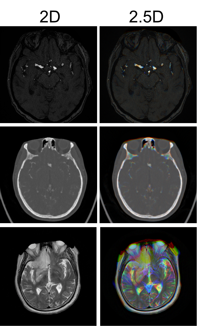\n\nAs can be seen in the examples, the images vary significantly because **we didn't standardize Z spacing**.\n\nI (@sersasj) spent 1-2 weeks experimenting with Z-axis resize, but results were consistently worse. Perhaps I was doing something wrong, but didn't have time to investigate further.\n\nWe were very reluctant to try 2.5D without proper Z-spacing resize (in my mind didn’t seem a good idea - @sersasj). Nevertheless, the 2.5D approach even without Z-resampling improved results by 0.02+ in CV.\n\n### **Training Configuration**\n\nData Sampling Strategy:\n\nFor negative samples we took 10 evenly sampled slices per series.\n\nExample: For a 100-slice series → slices [1, 11, 22, 33, 44, 56, 67, 78, 89, 99]\n\nFor positive samples we used all slices containing annotations\n\n### **YOLO with timm/tf_efficientnetv2_s Backbone**\n\n```yaml\nbatch_size: 16\nepochs: 50\nmixup: 0.4\nmosaic: 0.4\ndrop_path_rate: 0.2 \ncls_loss: 1.0\noptimizer: AdamW\nmomentum: 0.9\nlearning_rate: auto \n```\n\n### **YOLOv11m**\n\n```yaml\nbatch_size: 32\nepochs: 80\nmixup: 0.4\nmosaic: 0.4\ndroput: 0.3\ncls_loss: 1.0\noptimizer: AdamW\nmomentum: 0.9\nlearning_rate: auto \n```\n\nWe also modified the fitness function to include auc metric and prioritize mAP@50.\n\n```python\nfitness = 0.5 × mAP@50 + 0.25 × mAP@50-95 + 0.25 × mAUC\n\n```\n\nDid this help? Maybe a little. In the [BYU competition](https://www.kaggle.com/competitions/byu-locating-bacterial-flagellar-motors-2025/writeups/sergio-alvarez-paradox-17th-place-solution-ultraly), we had already found that prioritizing mAP@50 over the Ultralytics standard 1.0×mAP@50-95 gave better results.\n\nAdding AUC seemed like a good idea at the time since it's the competition metric, but we didn't investigate thoroughly whether it significantly improved performance. It's possible the benefit was marginal, but we kept it for consistency.\n\n**Training Hardware and Time**\n\n| Hardware Setup | GPU | CPU | RAM | Time per Fold | Total (5 folds) |\n| --- | --- | --- | --- | --- | --- |\n| @sersasj | RTX 3090 | Intel Core i5-12400F (12) @ 4.4GHz | 32GB | 4-5 hours | ~24 hours |\n| @iamparadox | RTX 4090 | AMD Ryzen 9 7950X (32) @ 5.883GHz | 64GB | ~2 hours | ~10 hours |\n\n### Inference\n\nFor inference, we sort DICOM slices by spatial position (SliceLocation → ImagePositionPatient → InstanceNumber), create 2.5D triplets for slices 1 to N-1\nRun batch inference across both models, extract max confidence per class and use max(localization_confidences) as overall aneurysm presence probability\nThe process can be observed in the gif below:\n.gif?generation=1761065820372307&alt=media)\n\n### Cross-Validation Scores\n\nfolds were stratified using `MultilabelStratifiedKFold` to ensure balanced distribution across:\n\n- Aneurysm presence\n- All 13 vessel locations\n- Modality\n\n### **YOLO11m 2.5D Results**\n\n| Fold | loc_macro_auc | cls_auc | combined_mean |\n| --- | --- | --- | --- |\n| fold0 | 0.8184 | 0.7549 | 0.7867 |\n| fold1 | 0.8114 | 0.7897 | 0.8005 |\n| fold2 | 0.8134 | 0.7827 | 0.7981 |\n| fold3 | 0.8162 | 0.7872 | 0.8017 |\n| fold4 | 0.8540 | 0.8281 | 0.8410 |\n| **Average** | **0.8227** | **0.7885** | **0.8056** |\n\n### **EfficientNetV2-S 2.5D Results**\n\n| Fold | loc_macro_auc | cls_auc | combined_mean |\n| --- | --- | --- | --- |\n| fold0 | 0.7978 | 0.7790 | 0.7884 |\n| fold1 | 0.8159 | 0.8269 | 0.8214 |\n| fold2 | 0.8155 | 0.7921 | 0.8038 |\n| fold3 | 0.8153 | 0.7907 | 0.8030 |\n| fold4 | 0.8499 | 0.8560 | 0.8529 |\n| **Average** | **0.8189** | **0.8090** | **0.8139** |\n\n### **Ensemble Results**\n\n| Fold | loc_macro_auc | cls_auc | combined_mean |\n| --- | --- | --- | --- |\n| fold0 | 0.8393 | 0.7849 | 0.8121 |\n| fold1 | 0.8330 | 0.8291 | 0.8310 |\n| fold2 | 0.8399 | 0.8135 | 0.8267 |\n| fold3 | 0.8370 | 0.8093 | 0.8232 |\n| fold4 | 0.8738 | 0.8620 | 0.8679 |\n| **Average** | **0.8446** | **0.8198** | **0.8322** |\n\n## What did not work:\n\nIn the initial stages of YOLO development @sersasj created an ensemble with 3xYolo11m and 0.69LB [EfficientNetB2 public notebook](https://www.kaggle.com/code/yosukeyama/rsna2025-32ch-img-infer-lb-0-69-share). That gave us a score of 0.78 LB and put us in the top 3 in early stages of competition\n\nAfter a bit of probing the leaderboard, @iamparadox found out that YOLO's aneurysm classification AUROC was very low (around ~0.58). Then we started to develop models that would complement YOLO and boost the aneurysm classification AUROC. (We later discovered that the poor results of early YOLO development were due to an insufficient amount of negative samples in training.)\n\nOne of the class of models that we used was 2.5D models that just detects the presence of aneurysm in the given series with auxiliary segmentation head. These models were inspired by https://www.kaggle.com/code/hengck23/3d-unet-using-2d-image-encoder. These models in combination with yolo11m gave us a LB of 0.80. \n\nThese models then became obsolete when we merged with @chihantsai, @atom1231.\n\nIn the BYU competition, our best-performing backbone was `timm/convnextv2_base.fcmae_ft_in22k_in1k`. However, in the current competition, training with half precision caused the loss to quickly become NaN. Based on our investigation, this appears to be a common issue with ConvNeXt architectures. We hypothesize that if trained in full precision, this backbone could achieve performance comparable to YOLO11m and `timm/tf_efficientnetv2_s.in21k_ft_in1k`. Unfortunately, we were unable to verify this due to time constraints.\n\nModifying the neck and head was also considered. From what we investigate with @tatamikenn [awesome reverse engineer notebook](https://www.kaggle.com/code/tatamikenn/reverse-engineering-yolo) P3 features appeared to be the most utilized. We conducted a quick test on a single fold, but results on validation were more or less the same so we decided to move on.\n\n.png?generation=1760534911466456&alt=media)\n\nWe also try to use our 3d segmentation result to [filter out invalid location prediction from yolo](https://www.kaggle.com/code/tom99763/rsna-iad-vessel-segmentation), but recall drops a lot.\nMoreover, we tried extracting patches using YOLO and applying wavelet and log-polar transforms to the patches before predicting their classes; however, [this approach ](https://www.kaggle.com/code/tom99763/yolos-phw-mip-lp-rsna-i) did not yield good results.\n\n## EfficientV2s + 3D-CenterNet (Flayer)\n\nThis is a highly **experimental project**, made with a lot of help from AI. We started with the popular “LB 0.69 Public Notebook” , reconstructed the entire **training pipeline and data preprocessing** from it, and then incorporated a **CenterNet-like mechanism to detect the center of the aneurysms**.\n\n### Model architecture\n\nWe adopt a **slice-wise 2D encoder + shallow 3D head** design:\n\n- **Encoder.** A 2D ImageNet-pretrained **EfficientNetV2-S** (`tf_efficientnetv2_s.in21k_ft_in1k`) from `timm` in *features_only* mode with the **penultimate** feature map (`out_indices = (1,-2)`).\n- **Auxiliary 2D head.**The intermediate feature map (early stage) is fed into a lightweight 2D convolutional head to produce per-slice auxiliary logits, which encourage the encoder to capture vessel-relevant spatial cues before 3D aggregation. The auxiliary head is supervised with slice-level targets to stabilize early-layer learning.\n- **2D→3D fusion.** Each volume `(B, C=1, D, H, W)` is **rearranged into `B·D` 2D slices**, encoded independently, then **reassembled** to `(B, C_feat, D, H′, W′)` before the 3D head. If the backbone expects 3 channels, single-channel inputs are channel-repeated.\n- **3D temporal head.** A lightweight head (Conv3d-BN-ReLU ×2, `base_channels`) aggregates signals across depth.\n- **Outputs.** Two 1×1×1 conv heads:\n - **Heatmap head:** `num_classes = 13` vessel locations (3D centerness maps)\n - **Offset head:** 3-channel sub-voxel offsets `(dz, dy, dx)`\n\n### Supervision targets\n\n- Place a **3D Gaussian** peak (stride-aware) at each annotated center on the class-specific heatmap.\n- Store **sub-voxel residual offsets** at the nearest grid cell and mark them with an **offset mask**.\n- Scale coordinates from the original series size to the current `(D, H, W)`; map to the output grid using `(stride_d=1, stride_h=stride_w=16)` so the output is `D × H/16 × W/16`.\n- Default **Gaussian σ = 0.2**.\n\n### Segmentation masks\nVessel masks are produced in physical space by training a 3D DynUNet on volumes resampled to 0.7 mm isotropic spacing. The provided voxel-level annotations of 13 vessel classes are merged into a single binary vessel mask for training. The resulting 3D masks are then converted to slice-wise 2D masks to supervise the auxiliary head.\n\n### Losses\n\nWe train with four terms and sum them with weights:\n\n- **CenterNet-style focal loss** (weight = 1.0) on heatmaps (α=2, β=4).\n- **L1 offset loss** (weight = 1.0) (only at valid center cells).\n- **BCE-with-logits classification loss** (weight = 1.0) from series-level logits .\n- **Auxiliary Dice & BCE loss** (weight = 0.5) on 2D auxiliary outputs when vessel segmentation masks are available; otherwise, it is set to zero, encouraging slice-wise feature consistency.\n\n### From voxelwise maps to series-level logits (for AUC & ensembling)\n\nGiven heatmap logits `H ∈ ℝ^{B×13×D×H′×W′}`:\n\n- **Per-class series logits:** spatial **max** over `(D, H′, W′)` for each of the 13 classes.\n- **Aneurysm Present (global) logit:** the **max over the 13** class logits.\n \n These **14 logits** drive the BCE loss and are exported for meta-ensembling.\n \n\n### Data pipeline & augmentations\n\n- **Input.** Precomputed `.npy` volumes; `(D,H,W)` expanded to `(1,D,H,W)`— here D = 64.\n- **Label scaling.** Rescale coordinates to current volume size; apply stride mapping for target grids.\n- **Augmentations.** A **shared 2D affine warp** per volume (same transform for all slices): random rotation, scale, translation; vertical flip available (off by default).\n- **Normalization.** Albumentations normalization → tensor conversion; channel repeat to 3-ch if needed.\n\n### Optimization & schedules\n\n- **Optimizer.** AdamW (LR=2e-4, weight decay=1e-5), **AMP** mixed precision, **grad clipping** (=1.0).\n- **LR schedule.** Default **CosineAnnealingLR** (`T_max = epochs`, `eta_min = 1e-6`); `StepLR` / `ReduceLROnPlateau` also supported.\n- **Checkpointing.** Best model selected by **mean AUC** on validation.\n\n### Training configuration\n\n- **Epochs:** 16\n- **Batch size:** 4 (train) / 2 (val)\n- **accumulate:**2\n- **Workers:** 16\n- **Strides:** depth `1`, lateral `16`\n- **Gaussian σ:** 0.2\n- **Backbone:** EfficientNetV2-S, `pretrained=True`, not frozen by default\n\n### Cross-validation & metrics\n\n- K-fold protocol driven by the training CSV split.\n- Compute **per-label ROC-AUC**, plus **mean** and **presence-weighted** AUC each epoch.\n- Scheduler stepping and best-by-mean-AUC saving per fold; final summary reports per-fold and average AUC.\n\n### **Flayer Results(without aux head)**\n\n| Fold | loc_macro_auc | cls_auc | combined_mean |\n| --- | --- | --- | --- |\n| fold0 | 0.7762 | 0.7747 | 0.7754 |\n| fold1 | 0.7676 | 0.8069 | 0.7873 |\n| fold2 | 0.7508 | 0.7892 | 0.7700 |\n| fold3 | 0.7553 | 0.7778 | 0.7666 |\n| fold4 | 0.7734 | 0.7758 | 0.7746 |\n| **Average** | **0.7647** | **0.7848** | **0.7748** |\n\n### **Flayer Results(with aux head)**\n\n| Fold | loc_macro_auc | cls_auc | combined_mean |\n| --- | --- | --- | --- |\n| fold0 | 0.7779 | 0.7991 | 0.7885 |\n| fold1 | 0.7828 | 0.7987 | 0.7908 |\n| fold2 | 0.7601 | 0.8051 | 0.7826 |\n| fold3 | 0.7683 | 0.7826 | 0.7755 |\n| fold4 | 0.7586 | 0.7954 | 0.7770 |\n| **Average** | **0.7695** | **0.7962** | **0.7829** |\n\n\n\n### Summary\n\n**Flayer** converts 2D EfficientNetV2-S slice features into 3D evidence maps with a light 3D head, supervises them using CenterNet-style heatmaps + offsets, and produces robust **14-logit** series-level predictions (including an aggregated *aneurysm present* logit) that plug cleanly into our stacked meta-classifier.\n\n## Meta Classifier\n\nWe designed a stacked ensemble architecture to integrate predictions from **YOLO11m**, **YOLO11-EffV2s**, and **EffV2s-3D-CenterNet** models. Specifically, each meta-classifier receives the concatenated predictions from all base models as input and produces final predictions for both **aneurysm presence** and **location-specific detection**. This setup enables the model to assess the presence of an aneurysm at a given location by considering predictions from all locations across all models, effectively capturing the ensemble’s collective reasoning about aneurysm presence.\n\n```python\n#for each fold_id\nmetadata = np.array([age, sex])\nX = np.concatenate([np.array([yolo11m_cls_preds[fold_id]]), yolo11m_loc_preds[fold_id],\n np.array([effv2s_cls_preds[fold_id]]), effv2s_loc_preds[fold_id],\n flayer_fold_preds[fold_id], metadata], axis=0)[None, :]\nlgb_pred = predict_prob_lgb(X, fold_id) #(14, )\nxgb_pred = predict_prob_xgb(X, fold_id)\ncat_pred = predict_prob_cat(X, fold_id)\n```\n\nWe experimented with two ensemble structures:\n\n- **Series:** A single YOLO prediction combined with one Flayer prediction is fed into the ensemble model to produce the final output. \n```\n(30 features, [yolo(14) + flayer(14) + meta(2)])\n```\n- **Parallel:** Two predictions from two YOLOs and one predictions from Flayer are processed in parallel and jointly used by the ensemble model to generate the final prediction. \n```\n(44 features, [yolo11m(14) + yolo_effnets(14)+ flayer(14) + meta(2)])\n```\n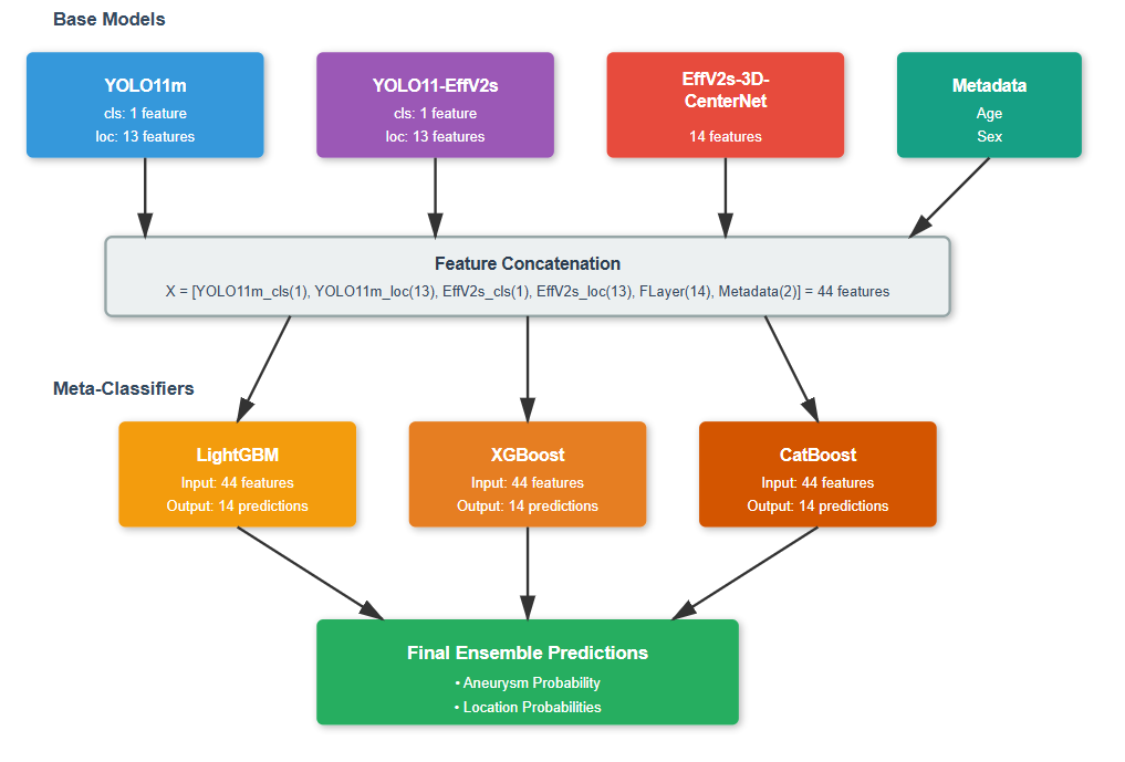\nThis comparison allows us to evaluate whether combining multiple feature streams in parallel provides additional complementary information beyond the sequential (series) configuration.\n\nWe found that combining predictions from different YOLO backbones and flayer in parallel provides better improvement than series in the ensemble CV score. This suggests that the GBDT effectively leverages each model’s perception of aneurysm presence across locations to make accurate judgments. We were unable to complete the 5-fold submission due to issues encountered on the final day. Therefore, we present here our final selected result, which is based on the average of 2 folds.\n\n| | Series | Parallel |\n| --- | --- | --- |\n| 5 folds CV (average) | 0.84 | **0.852** |\n| 5 folds CV (nelder-mead optimized) | 0.841 | **0.858** |\n| public score (average; 2 folds) | 0.83 | 0.83082 |\n| private score (average; 2 folds) | 0.81 | **0.8230** |\n\nWe’ve also tried Keypoint-Based Dual-Graph Predictor in [Tom’s BYU approach](https://www.kaggle.com/competitions/byu-locating-bacterial-flagellar-motors-2025/writeups/bias-vibes-trade-off-20th-place-solution-keypoint-) earlier and found it performed well in terms of ensemble CV performance. However, the YOLO-based feature extraction and preprocessing were too time-consuming and often led to timeouts. Therefore, we did not include this method in our final solution.\n\n## Codebase & Submission\n\nSubmission: \n* [**2x yolo + flayer + meta classifier (final ver)**](https://www.kaggle.com/code/tom99763/2x-yolo-flayer-meta-classifier-final-ver?scriptVersionId=267890122)\n\n* [kaggle models submission](https://www.kaggle.com/code/tom99763/9th-place-solution-rsna-iad)\n\nMeta classifier training: [**2x yolo + flayer meta training (final ver)**](https://www.kaggle.com/code/tom99763/2x-yolo-flayer-meta-training-final-ver)\n\nGithub: [9th-place-solution-yolo-RSNA-IAD](https://github.com/tom99763/9th-place-solution-yolo-RSNA-IAD)", "votes": 47 }, { "id": 3304634, "postDate": "2025-10-21T01:24:42.317Z", "content": "Flayer training code is updated in our github, also publish our kaggle Model
", "rawMarkdown": "Flayer training code is updated in [our github](https://github.com/tom99763/9th-place-solution-RSNA-IAD), also publish our [kaggle Model](https://www.kaggle.com/models/tom99763/9th-place-models-rsna-iad)", "votes": 1 }, { "id": 3302673, "postDate": "2025-10-16T09:09:10.200Z", "content": "I really like how kind this writing feels — congratulations!
", "rawMarkdown": "I really like how kind this writing feels — congratulations!" }, { "id": 3302586, "postDate": "2025-10-16T05:24:13.120Z", "content": "Hi, thanks for wonderful writeup. I have below questions.
\n\n\nDid you guys had any attempt with pure E2E 3D based solution?
\n
The biggest issues encountered with a pure 3D solution are insufficient computational power (compute) and excessively long training times. The CenterNet within the solution is a compromised/truncated 3D solution designed to mitigate the constraints of compute and time.
", "rawMarkdown": "> Did you guys had any attempt with pure E2E 3D based solution?\n\nThe biggest issues encountered with a pure 3D solution are insufficient computational power (compute) and excessively long training times. The CenterNet within the solution is a compromised/truncated 3D solution designed to mitigate the constraints of compute and time.", "votes": 1 }, { "id": 3302638, "postDate": "2025-10-16T08:08:12.570Z", "content": " specific reason GBDT the pipeline. I am correct Age + Sex metadata there test . (Was it just matter convinence?)\nThe reason of using meta-classifiers is that we noticed when predicting a class, aggregating predictions from other classes can give a significant CV boost. Therefore, we believe the predicted probabilities of other classes can also serve as useful clues for identifying aneurysms in a specific locations.
\nWe noticed that the sample test data contain Age and Sex, but after submitting, with or without meta data the didn’t change Leaderboard (LB) score much, while the cross-validation (CV) score showed a noticeable difference.
\nTherefore, we decided to keep Age and Sex features, assuming that some data in hidden test set also includes them.
Any motivation for D .D solution? (Was it of mixture of thick thin slices).\nIn the first month, we found that the 3D classifier approach tended to overfit easily, as representing each voxel along the channel dimension made the model prone to overfitting. However, depth context is crucial for detecting irregular structural changes that could indicate an aneurysm, and slice-wise predictions not having expected result here. We found that using 3 local adjancent depths as the channel dimension to represent each pixel outperforms other previous methods. This approach proved effective for YOLO in capturing anomaly locations based on slight depth structure changes and achieved better CV compared to YOLO models that takes processed single slices repeated along RGB channels.
", "rawMarkdown": "```\nAny specific reason for usage of GBDT in the pipeline. If I am correct Age + Sex metadata is not there for test set. (Was it just matter of convinence?)\n```\nThe reason of using meta-classifiers is that we noticed when predicting a class, aggregating predictions from other classes can give a significant CV boost. Therefore, we believe the predicted probabilities of other classes can also serve as useful clues for identifying aneurysms in a specific locations.\n\nWe noticed that the sample test data contain Age and Sex, but after submitting, with or without meta data the didn’t change Leaderboard (LB) score much, while the cross-validation (CV) score showed a noticeable difference.\nTherefore, we decided to keep Age and Sex features, assuming that some data in hidden test set also includes them.\n\n\n```\nAny motivation for 2D or 2.5D based solution? (Was it because of mixture of thick and thin slices).\n```\nIn the first month, we found that the 3D classifier approach tended to overfit easily, as representing each voxel along the channel dimension made the model prone to overfitting. However, depth context is crucial for detecting irregular structural changes that could indicate an aneurysm, and slice-wise predictions not having expected result here. We found that using 3 local adjancent depths as the channel dimension to represent each pixel outperforms other previous methods. This approach proved effective for YOLO in capturing anomaly locations based on slight depth structure changes and achieved better CV compared to YOLO models that takes processed single slices repeated along RGB channels.", "votes": 1, "replies": [ { "id": 3303104, "postDate": "2025-10-17T07:13:36.327Z", "content": "Thanks for additional information.
", "rawMarkdown": "Thanks for additional information. " } ] } ] }, { "id": 3302503, "postDate": "2025-10-16T01:10:49.220Z", "content": "Congratulations, very well done!
", "rawMarkdown": "Congratulations, very well done!" } ], "comments": [ { "id": 3304634, "author_name": "Tom", "author_url": "", "post_date": "2025-10-21T01:24:42.317000", "content": "Flayer training code is updated in our github, also publish our kaggle Model
", "votes": 1, "replies": [] }, { "id": 3302673, "author_name": "doheon114", "author_url": "", "post_date": "2025-10-16T09:09:10.200000", "content": "I really like how kind this writing feels — congratulations!
", "votes": 0, "replies": [] }, { "id": 3302586, "author_name": "Ujjwal Pandey", "author_url": "", "post_date": "2025-10-16T05:24:13.120000", "content": "Hi, thanks for wonderful writeup. I have below questions.
\n\n\nDid you guys had any attempt with pure E2E 3D based solution?
\n
The biggest issues encountered with a pure 3D solution are insufficient computational power (compute) and excessively long training times. The CenterNet within the solution is a compromised/truncated 3D solution designed to mitigate the constraints of compute and time.
", "votes": 1, "replies": [] }, { "id": 3302638, "author_name": "Tom", "author_url": "", "post_date": "2025-10-16T08:08:12.570000", "content": " specific reason GBDT the pipeline. I am correct Age + Sex metadata there test . (Was it just matter convinence?)\nThe reason of using meta-classifiers is that we noticed when predicting a class, aggregating predictions from other classes can give a significant CV boost. Therefore, we believe the predicted probabilities of other classes can also serve as useful clues for identifying aneurysms in a specific locations.
\nWe noticed that the sample test data contain Age and Sex, but after submitting, with or without meta data the didn’t change Leaderboard (LB) score much, while the cross-validation (CV) score showed a noticeable difference.
\nTherefore, we decided to keep Age and Sex features, assuming that some data in hidden test set also includes them.
Any motivation for D .D solution? (Was it of mixture of thick thin slices).\nIn the first month, we found that the 3D classifier approach tended to overfit easily, as representing each voxel along the channel dimension made the model prone to overfitting. However, depth context is crucial for detecting irregular structural changes that could indicate an aneurysm, and slice-wise predictions not having expected result here. We found that using 3 local adjancent depths as the channel dimension to represent each pixel outperforms other previous methods. This approach proved effective for YOLO in capturing anomaly locations based on slight depth structure changes and achieved better CV compared to YOLO models that takes processed single slices repeated along RGB channels.
", "votes": 1, "replies": [ { "id": 3303104, "author_name": "Ujjwal Pandey", "author_url": "", "post_date": "2025-10-17T07:13:36.327000", "content": "Thanks for additional information.
", "votes": 0, "replies": [] } ] } ] }, { "id": 3302503, "author_name": "Satwik", "author_url": "", "post_date": "2025-10-16T01:10:49.220000", "content": "Congratulations, very well done!
", "votes": 0, "replies": [] } ], "raw_markdown_by_id": { "3302294": "## Acknowledgement\n\nFirst, we thank the competition hosts @evancalabrese, @shosys and every person involved from RSNA in data preparation and competition related process, and Kaggle staff for organizing this competition. \n\nBelow, we introduce the solution of team **Vibes and Genius Trade-Off** -- @tom99763, @sersasj, @iamparadox, @chihantsai, @atom1231!\n\n**TL;DR**\n\nOur solution combines three complementary approaches:\n\n- YOLO 2.5D with different backbones. Derived from [BYU competition](https://www.kaggle.com/competitions/byu-locating-bacterial-flagellar-motors-2025/writeups/sergio-alvarez-paradox-17th-place-solution-ultraly)\n- 3D CenterNet with 2D Effv2s extractor.\n- Meta-classifiers (LightGBM, XGBoost, CatBoost)\n\nThe final probabilities are obtained by averaging the outputs of the YOLO 2.5D models, 3D CenterNet with 2D Effv2s extractor and the three meta-classifiers.\n\nHere is the diagram of our approach.\n\n\nWe used two different variations of YOLO:\n\n1. **YOLOv11m** - The standard YOLO11 medium model from Ultralytcs\n2. **Custom YOLO with timm backbone** - YOLO architecture with `timm/tf_efficientnetv2_s.in21k_ft_in1k` as the backbone\n\nFor details about the YOLO+timm customization, please refer to the [BYU writeup](https://www.kaggle.com/competitions/byu-locating-bacterial-flagellar-motors-2025/writeups/sergio-alvarez-paradox-17th-place-solution-ultraly).\n\nWe treated each of the **13 vessel locations as separate bounding box classes**:\n\n- Left/Right Infraclinoid Internal Carotid Artery\n- Left/Right Supraclinoid Internal Carotid Artery\n- Left/Right Middle Cerebral Artery\n- Anterior Communicating Artery\n- Left/Right Anterior Cerebral Artery\n- Left/Right Posterior Communicating Artery\n- Basilar Tip\n- Other Posterior Circulation\n\n### **2.5D Strategy**\n\nImages were resized to 512×512, normalized with min-max and converted to 2.5D variation:\n\n`R (Red channel) = slice i-1\nG (Green channel) = slice i\nB (Blue channel) = slice i+1`\n\nThe figure below shows examples of slices in 2D vs 2.5D variation:\n\n\n\nAs can be seen in the examples, the images vary significantly because **we didn't standardize Z spacing**.\n\nI (@sersasj) spent 1-2 weeks experimenting with Z-axis resize, but results were consistently worse. Perhaps I was doing something wrong, but didn't have time to investigate further.\n\nWe were very reluctant to try 2.5D without proper Z-spacing resize (in my mind didn’t seem a good idea - @sersasj). Nevertheless, the 2.5D approach even without Z-resampling improved results by 0.02+ in CV.\n\n### **Training Configuration**\n\nData Sampling Strategy:\n\nFor negative samples we took 10 evenly sampled slices per series.\n\nExample: For a 100-slice series → slices [1, 11, 22, 33, 44, 56, 67, 78, 89, 99]\n\nFor positive samples we used all slices containing annotations\n\n### **YOLO with timm/tf_efficientnetv2_s Backbone**\n\n```yaml\nbatch_size: 16\nepochs: 50\nmixup: 0.4\nmosaic: 0.4\ndrop_path_rate: 0.2 \ncls_loss: 1.0\noptimizer: AdamW\nmomentum: 0.9\nlearning_rate: auto \n```\n\n### **YOLOv11m**\n\n```yaml\nbatch_size: 32\nepochs: 80\nmixup: 0.4\nmosaic: 0.4\ndroput: 0.3\ncls_loss: 1.0\noptimizer: AdamW\nmomentum: 0.9\nlearning_rate: auto \n```\n\nWe also modified the fitness function to include auc metric and prioritize mAP@50.\n\n```python\nfitness = 0.5 × mAP@50 + 0.25 × mAP@50-95 + 0.25 × mAUC\n\n```\n\nDid this help? Maybe a little. In the [BYU competition](https://www.kaggle.com/competitions/byu-locating-bacterial-flagellar-motors-2025/writeups/sergio-alvarez-paradox-17th-place-solution-ultraly), we had already found that prioritizing mAP@50 over the Ultralytics standard 1.0×mAP@50-95 gave better results.\n\nAdding AUC seemed like a good idea at the time since it's the competition metric, but we didn't investigate thoroughly whether it significantly improved performance. It's possible the benefit was marginal, but we kept it for consistency.\n\n**Training Hardware and Time**\n\n| Hardware Setup | GPU | CPU | RAM | Time per Fold | Total (5 folds) |\n| --- | --- | --- | --- | --- | --- |\n| @sersasj | RTX 3090 | Intel Core i5-12400F (12) @ 4.4GHz | 32GB | 4-5 hours | ~24 hours |\n| @iamparadox | RTX 4090 | AMD Ryzen 9 7950X (32) @ 5.883GHz | 64GB | ~2 hours | ~10 hours |\n\n### Inference\n\nFor inference, we sort DICOM slices by spatial position (SliceLocation → ImagePositionPatient → InstanceNumber), create 2.5D triplets for slices 1 to N-1\nRun batch inference across both models, extract max confidence per class and use max(localization_confidences) as overall aneurysm presence probability\nThe process can be observed in the gif below:\n.gif?generation=1761065820372307&alt=media)\n\n### Cross-Validation Scores\n\nfolds were stratified using `MultilabelStratifiedKFold` to ensure balanced distribution across:\n\n- Aneurysm presence\n- All 13 vessel locations\n- Modality\n\n### **YOLO11m 2.5D Results**\n\n| Fold | loc_macro_auc | cls_auc | combined_mean |\n| --- | --- | --- | --- |\n| fold0 | 0.8184 | 0.7549 | 0.7867 |\n| fold1 | 0.8114 | 0.7897 | 0.8005 |\n| fold2 | 0.8134 | 0.7827 | 0.7981 |\n| fold3 | 0.8162 | 0.7872 | 0.8017 |\n| fold4 | 0.8540 | 0.8281 | 0.8410 |\n| **Average** | **0.8227** | **0.7885** | **0.8056** |\n\n### **EfficientNetV2-S 2.5D Results**\n\n| Fold | loc_macro_auc | cls_auc | combined_mean |\n| --- | --- | --- | --- |\n| fold0 | 0.7978 | 0.7790 | 0.7884 |\n| fold1 | 0.8159 | 0.8269 | 0.8214 |\n| fold2 | 0.8155 | 0.7921 | 0.8038 |\n| fold3 | 0.8153 | 0.7907 | 0.8030 |\n| fold4 | 0.8499 | 0.8560 | 0.8529 |\n| **Average** | **0.8189** | **0.8090** | **0.8139** |\n\n### **Ensemble Results**\n\n| Fold | loc_macro_auc | cls_auc | combined_mean |\n| --- | --- | --- | --- |\n| fold0 | 0.8393 | 0.7849 | 0.8121 |\n| fold1 | 0.8330 | 0.8291 | 0.8310 |\n| fold2 | 0.8399 | 0.8135 | 0.8267 |\n| fold3 | 0.8370 | 0.8093 | 0.8232 |\n| fold4 | 0.8738 | 0.8620 | 0.8679 |\n| **Average** | **0.8446** | **0.8198** | **0.8322** |\n\n## What did not work:\n\nIn the initial stages of YOLO development @sersasj created an ensemble with 3xYolo11m and 0.69LB [EfficientNetB2 public notebook](https://www.kaggle.com/code/yosukeyama/rsna2025-32ch-img-infer-lb-0-69-share). That gave us a score of 0.78 LB and put us in the top 3 in early stages of competition\n\nAfter a bit of probing the leaderboard, @iamparadox found out that YOLO's aneurysm classification AUROC was very low (around ~0.58). Then we started to develop models that would complement YOLO and boost the aneurysm classification AUROC. (We later discovered that the poor results of early YOLO development were due to an insufficient amount of negative samples in training.)\n\nOne of the class of models that we used was 2.5D models that just detects the presence of aneurysm in the given series with auxiliary segmentation head. These models were inspired by https://www.kaggle.com/code/hengck23/3d-unet-using-2d-image-encoder. These models in combination with yolo11m gave us a LB of 0.80. \n\nThese models then became obsolete when we merged with @chihantsai, @atom1231.\n\nIn the BYU competition, our best-performing backbone was `timm/convnextv2_base.fcmae_ft_in22k_in1k`. However, in the current competition, training with half precision caused the loss to quickly become NaN. Based on our investigation, this appears to be a common issue with ConvNeXt architectures. We hypothesize that if trained in full precision, this backbone could achieve performance comparable to YOLO11m and `timm/tf_efficientnetv2_s.in21k_ft_in1k`. Unfortunately, we were unable to verify this due to time constraints.\n\nModifying the neck and head was also considered. From what we investigate with @tatamikenn [awesome reverse engineer notebook](https://www.kaggle.com/code/tatamikenn/reverse-engineering-yolo) P3 features appeared to be the most utilized. We conducted a quick test on a single fold, but results on validation were more or less the same so we decided to move on.\n\n.png?generation=1760534911466456&alt=media)\n\nWe also try to use our 3d segmentation result to [filter out invalid location prediction from yolo](https://www.kaggle.com/code/tom99763/rsna-iad-vessel-segmentation), but recall drops a lot.\nMoreover, we tried extracting patches using YOLO and applying wavelet and log-polar transforms to the patches before predicting their classes; however, [this approach ](https://www.kaggle.com/code/tom99763/yolos-phw-mip-lp-rsna-i) did not yield good results.\n\n## EfficientV2s + 3D-CenterNet (Flayer)\n\nThis is a highly **experimental project**, made with a lot of help from AI. We started with the popular “LB 0.69 Public Notebook” , reconstructed the entire **training pipeline and data preprocessing** from it, and then incorporated a **CenterNet-like mechanism to detect the center of the aneurysms**.\n\n### Model architecture\n\nWe adopt a **slice-wise 2D encoder + shallow 3D head** design:\n\n- **Encoder.** A 2D ImageNet-pretrained **EfficientNetV2-S** (`tf_efficientnetv2_s.in21k_ft_in1k`) from `timm` in *features_only* mode with the **penultimate** feature map (`out_indices = (1,-2)`).\n- **Auxiliary 2D head.**The intermediate feature map (early stage) is fed into a lightweight 2D convolutional head to produce per-slice auxiliary logits, which encourage the encoder to capture vessel-relevant spatial cues before 3D aggregation. The auxiliary head is supervised with slice-level targets to stabilize early-layer learning.\n- **2D→3D fusion.** Each volume `(B, C=1, D, H, W)` is **rearranged into `B·D` 2D slices**, encoded independently, then **reassembled** to `(B, C_feat, D, H′, W′)` before the 3D head. If the backbone expects 3 channels, single-channel inputs are channel-repeated.\n- **3D temporal head.** A lightweight head (Conv3d-BN-ReLU ×2, `base_channels`) aggregates signals across depth.\n- **Outputs.** Two 1×1×1 conv heads:\n - **Heatmap head:** `num_classes = 13` vessel locations (3D centerness maps)\n - **Offset head:** 3-channel sub-voxel offsets `(dz, dy, dx)`\n\n### Supervision targets\n\n- Place a **3D Gaussian** peak (stride-aware) at each annotated center on the class-specific heatmap.\n- Store **sub-voxel residual offsets** at the nearest grid cell and mark them with an **offset mask**.\n- Scale coordinates from the original series size to the current `(D, H, W)`; map to the output grid using `(stride_d=1, stride_h=stride_w=16)` so the output is `D × H/16 × W/16`.\n- Default **Gaussian σ = 0.2**.\n\n### Segmentation masks\nVessel masks are produced in physical space by training a 3D DynUNet on volumes resampled to 0.7 mm isotropic spacing. The provided voxel-level annotations of 13 vessel classes are merged into a single binary vessel mask for training. The resulting 3D masks are then converted to slice-wise 2D masks to supervise the auxiliary head.\n\n### Losses\n\nWe train with four terms and sum them with weights:\n\n- **CenterNet-style focal loss** (weight = 1.0) on heatmaps (α=2, β=4).\n- **L1 offset loss** (weight = 1.0) (only at valid center cells).\n- **BCE-with-logits classification loss** (weight = 1.0) from series-level logits .\n- **Auxiliary Dice & BCE loss** (weight = 0.5) on 2D auxiliary outputs when vessel segmentation masks are available; otherwise, it is set to zero, encouraging slice-wise feature consistency.\n\n### From voxelwise maps to series-level logits (for AUC & ensembling)\n\nGiven heatmap logits `H ∈ ℝ^{B×13×D×H′×W′}`:\n\n- **Per-class series logits:** spatial **max** over `(D, H′, W′)` for each of the 13 classes.\n- **Aneurysm Present (global) logit:** the **max over the 13** class logits.\n \n These **14 logits** drive the BCE loss and are exported for meta-ensembling.\n \n\n### Data pipeline & augmentations\n\n- **Input.** Precomputed `.npy` volumes; `(D,H,W)` expanded to `(1,D,H,W)`— here D = 64.\n- **Label scaling.** Rescale coordinates to current volume size; apply stride mapping for target grids.\n- **Augmentations.** A **shared 2D affine warp** per volume (same transform for all slices): random rotation, scale, translation; vertical flip available (off by default).\n- **Normalization.** Albumentations normalization → tensor conversion; channel repeat to 3-ch if needed.\n\n### Optimization & schedules\n\n- **Optimizer.** AdamW (LR=2e-4, weight decay=1e-5), **AMP** mixed precision, **grad clipping** (=1.0).\n- **LR schedule.** Default **CosineAnnealingLR** (`T_max = epochs`, `eta_min = 1e-6`); `StepLR` / `ReduceLROnPlateau` also supported.\n- **Checkpointing.** Best model selected by **mean AUC** on validation.\n\n### Training configuration\n\n- **Epochs:** 16\n- **Batch size:** 4 (train) / 2 (val)\n- **accumulate:**2\n- **Workers:** 16\n- **Strides:** depth `1`, lateral `16`\n- **Gaussian σ:** 0.2\n- **Backbone:** EfficientNetV2-S, `pretrained=True`, not frozen by default\n\n### Cross-validation & metrics\n\n- K-fold protocol driven by the training CSV split.\n- Compute **per-label ROC-AUC**, plus **mean** and **presence-weighted** AUC each epoch.\n- Scheduler stepping and best-by-mean-AUC saving per fold; final summary reports per-fold and average AUC.\n\n### **Flayer Results(without aux head)**\n\n| Fold | loc_macro_auc | cls_auc | combined_mean |\n| --- | --- | --- | --- |\n| fold0 | 0.7762 | 0.7747 | 0.7754 |\n| fold1 | 0.7676 | 0.8069 | 0.7873 |\n| fold2 | 0.7508 | 0.7892 | 0.7700 |\n| fold3 | 0.7553 | 0.7778 | 0.7666 |\n| fold4 | 0.7734 | 0.7758 | 0.7746 |\n| **Average** | **0.7647** | **0.7848** | **0.7748** |\n\n### **Flayer Results(with aux head)**\n\n| Fold | loc_macro_auc | cls_auc | combined_mean |\n| --- | --- | --- | --- |\n| fold0 | 0.7779 | 0.7991 | 0.7885 |\n| fold1 | 0.7828 | 0.7987 | 0.7908 |\n| fold2 | 0.7601 | 0.8051 | 0.7826 |\n| fold3 | 0.7683 | 0.7826 | 0.7755 |\n| fold4 | 0.7586 | 0.7954 | 0.7770 |\n| **Average** | **0.7695** | **0.7962** | **0.7829** |\n\n\n\n### Summary\n\n**Flayer** converts 2D EfficientNetV2-S slice features into 3D evidence maps with a light 3D head, supervises them using CenterNet-style heatmaps + offsets, and produces robust **14-logit** series-level predictions (including an aggregated *aneurysm present* logit) that plug cleanly into our stacked meta-classifier.\n\n## Meta Classifier\n\nWe designed a stacked ensemble architecture to integrate predictions from **YOLO11m**, **YOLO11-EffV2s**, and **EffV2s-3D-CenterNet** models. Specifically, each meta-classifier receives the concatenated predictions from all base models as input and produces final predictions for both **aneurysm presence** and **location-specific detection**. This setup enables the model to assess the presence of an aneurysm at a given location by considering predictions from all locations across all models, effectively capturing the ensemble’s collective reasoning about aneurysm presence.\n\n```python\n#for each fold_id\nmetadata = np.array([age, sex])\nX = np.concatenate([np.array([yolo11m_cls_preds[fold_id]]), yolo11m_loc_preds[fold_id],\n np.array([effv2s_cls_preds[fold_id]]), effv2s_loc_preds[fold_id],\n flayer_fold_preds[fold_id], metadata], axis=0)[None, :]\nlgb_pred = predict_prob_lgb(X, fold_id) #(14, )\nxgb_pred = predict_prob_xgb(X, fold_id)\ncat_pred = predict_prob_cat(X, fold_id)\n```\n\nWe experimented with two ensemble structures:\n\n- **Series:** A single YOLO prediction combined with one Flayer prediction is fed into the ensemble model to produce the final output. \n```\n(30 features, [yolo(14) + flayer(14) + meta(2)])\n```\n- **Parallel:** Two predictions from two YOLOs and one predictions from Flayer are processed in parallel and jointly used by the ensemble model to generate the final prediction. \n```\n(44 features, [yolo11m(14) + yolo_effnets(14)+ flayer(14) + meta(2)])\n```\n\nThis comparison allows us to evaluate whether combining multiple feature streams in parallel provides additional complementary information beyond the sequential (series) configuration.\n\nWe found that combining predictions from different YOLO backbones and flayer in parallel provides better improvement than series in the ensemble CV score. This suggests that the GBDT effectively leverages each model’s perception of aneurysm presence across locations to make accurate judgments. We were unable to complete the 5-fold submission due to issues encountered on the final day. Therefore, we present here our final selected result, which is based on the average of 2 folds.\n\n| | Series | Parallel |\n| --- | --- | --- |\n| 5 folds CV (average) | 0.84 | **0.852** |\n| 5 folds CV (nelder-mead optimized) | 0.841 | **0.858** |\n| public score (average; 2 folds) | 0.83 | 0.83082 |\n| private score (average; 2 folds) | 0.81 | **0.8230** |\n\nWe’ve also tried Keypoint-Based Dual-Graph Predictor in [Tom’s BYU approach](https://www.kaggle.com/competitions/byu-locating-bacterial-flagellar-motors-2025/writeups/bias-vibes-trade-off-20th-place-solution-keypoint-) earlier and found it performed well in terms of ensemble CV performance. However, the YOLO-based feature extraction and preprocessing were too time-consuming and often led to timeouts. Therefore, we did not include this method in our final solution.\n\n## Codebase & Submission\n\nSubmission: \n* [**2x yolo + flayer + meta classifier (final ver)**](https://www.kaggle.com/code/tom99763/2x-yolo-flayer-meta-classifier-final-ver?scriptVersionId=267890122)\n\n* [kaggle models submission](https://www.kaggle.com/code/tom99763/9th-place-solution-rsna-iad)\n\nMeta classifier training: [**2x yolo + flayer meta training (final ver)**](https://www.kaggle.com/code/tom99763/2x-yolo-flayer-meta-training-final-ver)\n\nGithub: [9th-place-solution-yolo-RSNA-IAD](https://github.com/tom99763/9th-place-solution-yolo-RSNA-IAD)", "3304634": "Flayer training code is updated in [our github](https://github.com/tom99763/9th-place-solution-RSNA-IAD), also publish our [kaggle Model](https://www.kaggle.com/models/tom99763/9th-place-models-rsna-iad)", "3302673": "I really like how kind this writing feels — congratulations!", "3302586": "Hi, thanks for wonderful writeup. I have below questions.\n\n1. Did you guys considred trying out reorientation or resampling of the niftii volume in pre-processing pipeline?\n2. Any specific reason for usage of GBDT in the pipeline. If I am correct Age + Sex metadata is not there for test set. (Was it just matter of convinence?)\n2. Any motivation for 2D or 2.5D based solution? (Was it because of mixture of thick and thin slices).\n3. Did you guys had any attempt with pure E2E 3D based solution?", "3302503": "Congratulations, very well done!" } }