{"cells":[{"metadata":{},"cell_type":"markdown","source":"## Chest Abnormality Detection with YOLO-v3\n\n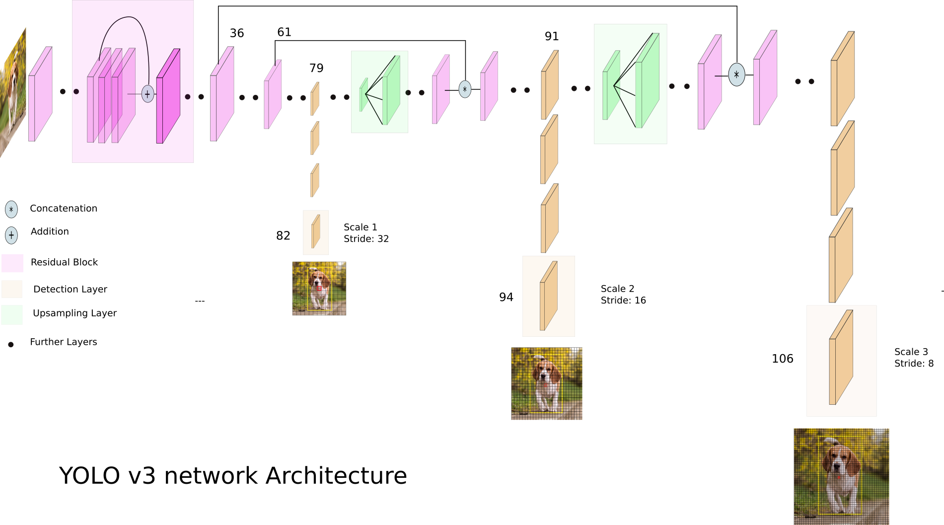"},{"metadata":{},"cell_type":"markdown","source":"## Credits\n\nPlease go and visit these below mentioned notebooks and support their works. Without the help of the below mentioned notebooks, it would have been much difficult for me to approach the solution.\n\n1. [VinBigData-CXR-AD YOLOv5 14 Class [train]](https://www.kaggle.com/awsaf49/vinbigdata-cxr-ad-yolov5-14-class-train)\n\n2. [VinBigData-CXR-AD YOLOv5 14 Class [infer]](https://www.kaggle.com/awsaf49/vinbigdata-cxr-ad-yolov5-14-class-infer)\n\n3. [VinBigData: Process and resize to PNG (1024x1024)](https://www.kaggle.com/xhlulu/vinbigdata-process-and-resize-to-png-1024x1024)\n\n4. [VinBigData: Process and resize to image](https://www.kaggle.com/xhlulu/vinbigdata-process-and-resize-to-image)\n\n5. [chest generate training folds](https://www.kaggle.com/abhishek/chest-generate-training-folds)\n\n6. video -> [Train custom object detection model with YOLO V5](https://youtu.be/NU9Xr_NYslo) by [Abhishek Thakur](https://www.kaggle.com/abhishek)"},{"metadata":{},"cell_type":"markdown","source":"## My Previous work on VinBigData Chest X-ray Abnormalities Detection\n\n1. [Chest X-ray Abnormalities Detection](https://www.kaggle.com/basu369victor/chest-x-ray-abnormalities-detection)\n\nTopics utilized in the above notebook.\n * FasterRCNN from torchvision\n * Uses Resnet50+FPN backbone\n * Normalization of the X-ray images\n * Visualization of Model performance over validation images\n\n2. [Chest X-ray Abnormalities Detection(Submission)](https://www.kaggle.com/basu369victor/chest-x-ray-abnormalities-detection-submission)\n\n\n**If you find my previous notebooks informative and useful please do support my work by upvoting them and also let me know your opinions in the comments**."},{"metadata":{"trusted":true,"_kg_hide-output":true},"cell_type":"code","source":"!pip install bbox-visualizer","execution_count":null,"outputs":[]},{"metadata":{"_uuid":"8f2839f25d086af736a60e9eeb907d3b93b6e0e5","_cell_guid":"b1076dfc-b9ad-4769-8c92-a6c4dae69d19","trusted":true,"scrolled":true},"cell_type":"code","source":"import numpy as np\nimport pandas as pd\nfrom glob import glob\nimport shutil, os\n\nimport matplotlib.pyplot as plt\nimport seaborn as sns\nimport bbox_visualizer as bbv\n\nfrom sklearn.model_selection import GroupKFold\nfrom tqdm.notebook import tqdm\n\nimport cv2","execution_count":null,"outputs":[]},{"metadata":{"_uuid":"d629ff2d2480ee46fbb7e2d37f6b5fab8052498a","_cell_guid":"79c7e3d0-c299-4dcb-8224-4455121ee9b0","trusted":true,"scrolled":true},"cell_type":"code","source":"size = 512\nBASE_DIR = '../input/vinbigdata-chest-xray-abnormalities-detection/'\nif size == 512:\n External_DIR = '../input/vinbigdata'\nif size == 1024:\n External_DIR = '../input/vinbigdata-chest-xray-resized-png-1024x1024'","execution_count":null,"outputs":[]},{"metadata":{"trusted":true,"scrolled":true},"cell_type":"code","source":"train_df = pd.read_csv(os.path.join(BASE_DIR, \"train.csv\"))\ntrain_df.head()","execution_count":null,"outputs":[]},{"metadata":{"trusted":true,"scrolled":true},"cell_type":"code","source":"train_df = train_df[train_df.class_name!='No finding'].reset_index(drop=True)","execution_count":null,"outputs":[]},{"metadata":{"trusted":true,"scrolled":true},"cell_type":"code","source":"train_dim = pd.read_csv(os.path.join(External_DIR, \"train_meta.csv\"))\ntrain_dim.head()","execution_count":null,"outputs":[]},{"metadata":{"trusted":true,"scrolled":true},"cell_type":"code","source":"train = pd.merge(train_df, train_dim, on='image_id')\ntrain.head()","execution_count":null,"outputs":[]},{"metadata":{},"cell_type":"markdown","source":"## Pre-processing"},{"metadata":{"trusted":true,"scrolled":true},"cell_type":"code","source":"# reshaping the bounding-box w.r.t. the resized image\ntrain['x_min'] = train.apply(lambda row: (row.x_min)/row.dim1, axis = 1)*float(size)\ntrain['y_min'] = train.apply(lambda row: (row.y_min)/row.dim0, axis = 1)*float(size)\n\ntrain['x_max'] = train.apply(lambda row: (row.x_max)/row.dim1, axis =1)*float(size)\ntrain['y_max'] = train.apply(lambda row: (row.y_max)/row.dim0, axis =1)*float(size)\n\n# calculation x-mid, y-mid, width and hight of the bounding box for yolo\ntrain['x_mid'] = train.apply(lambda row: (row.x_max+row.x_min)/2, axis =1)\ntrain['y_mid'] = train.apply(lambda row: (row.y_max+row.y_min)/2, axis =1)\n\ntrain['w'] = train.apply(lambda row: (row.x_max-row.x_min), axis =1)\ntrain['h'] = train.apply(lambda row: (row.y_max-row.y_min), axis =1)\n\ntrain['x_mid'] /= float(size)\ntrain['y_mid'] /= float(size)\n\ntrain['w'] /= float(size)\ntrain['h'] /= float(size)\n\ntrain['area'] = train['w']*train['h']\ntrain.head()","execution_count":null,"outputs":[]},{"metadata":{"trusted":true,"scrolled":true},"cell_type":"code","source":"Kfold = GroupKFold(n_splits = 3)\ntrain['fold'] = -1\nfor fold, (train_idx, val_idx) in enumerate(Kfold.split(train, groups = train.image_id.values)):\n train.loc[val_idx, 'fold'] = fold\ntrain.head()","execution_count":null,"outputs":[]},{"metadata":{"trusted":true,"scrolled":true},"cell_type":"code","source":"fold_0 = 1\nfold_1 = 2\ntrain_files = []\nval_files = []\n\ntrain_files += list(train[train.fold==fold_0].image_id.unique())\nval_files += list(train[train.fold==fold_1].image_id.unique())\nlen(train_files), len(val_files)","execution_count":null,"outputs":[]},{"metadata":{},"cell_type":"markdown","source":"## Chest X-ray bounding bounding box visualization\n\nIf the image size is 1024, you could use the **visualize_plot** function to visualize x-rays with bounding boxes, but I would not recommend this in case of 512 or lower size images because of the low-quality plots in the final visualized result.
\nI have already created similar plots in my [Chest X-ray Abnormalities Detection](https://www.kaggle.com/basu369victor/chest-x-ray-abnormalities-detection) notebook, so you could go and check them out.\n"},{"metadata":{"trusted":true},"cell_type":"code","source":"def visualize_plot(idx):\n image = train_files[idx]\n records = train[train['image_id'] == image]\n boxes = np.array(records[['x_min','y_min','x_max','y_max']])\n \n labels = records.class_name\n sample = cv2.imread(os.path.join('/content','train',f'{image}.png'))\n img = sample.copy()\n plt.figure(figsize=(16, 16))\n for box,label in zip(boxes,labels):\n bbv.add_label(img, \n label, \n [int(round(box[0])), int(round(box[1])),int(round(box[2])), int(round(box[3]))], \n draw_bg=True,\n text_bg_color=(255,0,0),\n text_color=(0,0,0),\n )\n cv2.rectangle(img ,\n (int(round(box[0])), int(round(box[1]))),\n (int(round(box[2])), int(round(box[3]))),\n (255,0,0),\n 2)\n\n\n plt.imshow(img)","execution_count":null,"outputs":[]},{"metadata":{"trusted":true},"cell_type":"code","source":"#visualize_plot(0)","execution_count":null,"outputs":[]},{"metadata":{"trusted":true},"cell_type":"code","source":"#visualize_plot(12)","execution_count":null,"outputs":[]},{"metadata":{"trusted":true},"cell_type":"code","source":"#visualize_plot(24)","execution_count":null,"outputs":[]},{"metadata":{"trusted":true},"cell_type":"code","source":"#visualize_plot(30)","execution_count":null,"outputs":[]},{"metadata":{"trusted":true},"cell_type":"code","source":"#visualize_plot(62)","execution_count":null,"outputs":[]},{"metadata":{},"cell_type":"markdown","source":"## Directory Tree for YOLO"},{"metadata":{"trusted":true,"scrolled":true},"cell_type":"code","source":"os.makedirs('./vinbigdata/labels/train', exist_ok = True)\nos.makedirs('./vinbigdata/labels/val', exist_ok = True)\nos.makedirs('./vinbigdata/images/train', exist_ok = True)\nos.makedirs('./vinbigdata/images/val', exist_ok = True)","execution_count":null,"outputs":[]},{"metadata":{"trusted":true,"scrolled":true},"cell_type":"code","source":"TRAIN_LABELS_PATH = './vinbigdata/labels/train'\nVAL_LABELS_PATH = './vinbigdata/labels/val'\nTRAIN_IMAGES_PATH = './vinbigdata/images/train'\nVAL_IMAGES_PATH = './vinbigdata/images/val'\n\nfor file in tqdm(train_files):\n records = train[train['image_id'] == file]\n attributes = records[['class_id','x_mid','y_mid','w','h']].values\n attributes = np.array(attributes)\n np.savetxt(\n os.path.join(\n TRAIN_LABELS_PATH,\n f\"{file}.txt\"\n ),\n attributes,\n fmt = [\"%d\",\"%f\",\"%f\",\"%f\",\"%f\"]\n )\n shutil.copy(\n os.path.join(\n External_DIR,\n 'train',\n f\"{file}.png\" \n ), \n TRAIN_IMAGES_PATH\n )","execution_count":null,"outputs":[]},{"metadata":{"trusted":true,"scrolled":true},"cell_type":"code","source":"for file in tqdm(val_files):\n records = train[train['image_id'] == file]\n attributes = records[['class_id','x_mid','y_mid','w','h']]\n attributes = np.array(attributes)\n np.savetxt(\n os.path.join(\n VAL_LABELS_PATH,\n f\"{file}.txt\"\n ),\n attributes,\n fmt = [\"%d\",\"%f\",\"%f\",\"%f\",\"%f\"]\n )\n shutil.copy(\n os.path.join(\n External_DIR,\n 'train',\n f\"{file}.png\" \n ), \n VAL_IMAGES_PATH\n )","execution_count":null,"outputs":[]},{"metadata":{"trusted":true,"scrolled":true},"cell_type":"code","source":"class_ids, class_names = list(zip(*set(zip(train.class_id, train.class_name))))\nclasses = list(np.array(class_names)[np.argsort(class_ids)])\nclasses = list(map(lambda x: str(x), classes))\nclasses","execution_count":null,"outputs":[]},{"metadata":{"trusted":true,"scrolled":true},"cell_type":"code","source":"from os import listdir\nfrom os.path import isfile, join\nimport yaml\n\ncwd = './'\n\nwith open(join( cwd , 'train.txt'), 'w') as f:\n for path in glob('./vinbigdata/images/train/*'):\n f.write(path+'\\n')\n \nwith open(join( cwd , 'val.txt'), 'w') as f:\n for path in glob('./vinbigdata/images/val/*'):\n f.write(path+'\\n')\n\ndata = dict(\n train = '../train.txt',\n val = '../val.txt',\n nc = 14,\n names = classes\n )\n\nwith open(join( cwd , 'vinbigdata.yaml'), 'w') as outfile:\n yaml.dump(data, outfile, default_flow_style=False)\n \nf = open(join( cwd, 'vinbigdata.yaml'), 'r')\nprint('\\nyaml:')\nprint(f.read())","execution_count":null,"outputs":[]},{"metadata":{},"cell_type":"markdown","source":"## Explanation\n\nSo I was trying to approach this problem with [**Scaled YOLO-v4**](https://arxiv.org/pdf/2011.08036.pdf), but the approach did not go well, the recall score was pretty low and the model was not predicting the bounding box. My assumptions are that if the model was trained for many iterations or if the model parameters would have been tuned manually like iou_threshold, or convolution layer parameters the model would have worked fine.
\n\nNow, Yolo-v5 and Yolo-v4 are far better than Yolo-v3 then why did I go for Yolo-v3. Yolo-v5 for this problem has already been implemented in this notebook- [VinBigData-CXR-AD YOLOv5 14 Class [train]](https://www.kaggle.com/awsaf49/vinbigdata-cxr-ad-yolov5-14-class-train)\n, and I think the performance is really good. For Yolo-v4, I kept it for later experimentation. And with Yolo-v3 I tried because I was curious to know how an older methodology would work over a medical imaging scenario. \n\nAlso, I came across this research paper where YOLO-v2 with DenseNet201 in backend network has been used for chest x-ray abnormality detection, [Reproducibility of abnormality detection on chest radiographs using convolutional neural network in paired radiographs obtained within a short-term interval](https://www.nature.com/articles/s41598-020-74626-4). I think this research paper is pretty interesting and you could give it a look. The output layers of eDenseYOLO, which is You Only Look Once v2 with DenseNet201, were modified for improved robustness to the variable size of disease patterns. If the input resolution was 256 × 256, the feature map for the last layer was 8 × 8, 16 × 16, and 32 × 32 with skip connection."},{"metadata":{},"cell_type":"markdown","source":"## Implementation of Scaled YOLO-v4\n\n\nI have commented out the scaled Yolo implementation part because the final results were not promising, but you could give it a try in your side, and have promising and better solution over this problem."},{"metadata":{"_kg_hide-output":true,"trusted":true,"scrolled":false},"cell_type":"code","source":"#!git clone https://github.com/AlexeyAB/darknet\n#!wget https://github.com/AlexeyAB/darknet/releases/download/darknet_yolo_v4_pre/yolov4-csp.weights\n#!git clone -b yolov4-csp https://github.com/WongKinYiu/ScaledYOLOv4.git","execution_count":null,"outputs":[]},{"metadata":{"trusted":true},"cell_type":"code","source":"#!git clone https://github.com/JunnYu/mish-cuda.git\n#%cd mish-cuda\n#!python setup.py build install\n#%cd ..","execution_count":null,"outputs":[]},{"metadata":{"trusted":true},"cell_type":"code","source":"#!git clone https://github.com/WongKinYiu/ScaledYOLOv4.git\n#%cd ./ScaledYOLOv4/\n#!git checkout yolov4-csp","execution_count":null,"outputs":[]},{"metadata":{"trusted":true},"cell_type":"code","source":"#!python train.py --img 512 512 --batch-size 24 --epochs 20 --data ../vinbigdata.yaml --cfg yolov4-csp.cfg --weights ../yolov4-csp.weights --cache","execution_count":null,"outputs":[]},{"metadata":{},"cell_type":"markdown","source":"## Yolo V3"},{"metadata":{"trusted":true},"cell_type":"code","source":"!git clone https://github.com/ultralytics/yolov3.git\n%cd ./yolov3/\n!pip install -r requirements.txt","execution_count":null,"outputs":[]},{"metadata":{"trusted":true},"cell_type":"code","source":"!wget https://github.com/ultralytics/yolov3/releases/download/v9.1/yolov3.pt\n#!wget https://github.com/ultralytics/yolov3/releases/download/v9.1/yolov3-spp.pt\n#!wget https://github.com/ultralytics/yolov3/releases/download/v9.1/yolov3-tiny.pt","execution_count":null,"outputs":[]},{"metadata":{"trusted":true},"cell_type":"code","source":"!WANDB_MODE=\"dryrun\" python train.py --img {size} --batch-size 40 --epochs 60 --data ../vinbigdata.yaml --weights yolov3.pt","execution_count":null,"outputs":[]},{"metadata":{},"cell_type":"markdown","source":"## Yolo performance evaluation"},{"metadata":{"_kg_hide-output":true,"trusted":true},"cell_type":"code","source":"!pip install matplotlib==3.1.3\nimport matplotlib.pyplot as plt","execution_count":null,"outputs":[]},{"metadata":{"trusted":true},"cell_type":"code","source":"plt.figure(figsize=(30,15))\nplt.axis('off')\nplt.imshow(plt.imread('runs/train/exp/results.png'));","execution_count":null,"outputs":[]},{"metadata":{"trusted":true},"cell_type":"code","source":"plt.figure(figsize=(30,15))\nplt.axis('off')\nplt.imshow(plt.imread('runs/train/exp/precision_recall_curve.png'));","execution_count":null,"outputs":[]},{"metadata":{"trusted":true},"cell_type":"code","source":"plt.figure(figsize=(30,15))\nplt.axis('off')\nplt.imshow(plt.imread('./runs/train/exp/labels.jpg'));","execution_count":null,"outputs":[]},{"metadata":{"trusted":true},"cell_type":"code","source":"_, ax = plt.subplots(1, 2, figsize=(20, 20))\n\nax[0].imshow(plt.imread('runs/train/exp/test_batch0_labels.jpg'))\nax[1].imshow(plt.imread('runs/train/exp/test_batch0_pred.jpg'))\nax[0].title.set_text('Ground Truth')\nax[1].title.set_text('YOLO predictions')","execution_count":null,"outputs":[]},{"metadata":{"trusted":true},"cell_type":"code","source":"_, ax = plt.subplots(1, 2, figsize=(20, 20))\n\nax[0].imshow(plt.imread('runs/train/exp/test_batch1_labels.jpg'))\nax[1].imshow(plt.imread('runs/train/exp/test_batch1_pred.jpg'))\nax[0].title.set_text('Ground Truth')\nax[1].title.set_text('YOLO predictions')","execution_count":null,"outputs":[]},{"metadata":{"trusted":true},"cell_type":"code","source":"_, ax = plt.subplots(1, 2, figsize=(20, 20))\n\nax[0].imshow(plt.imread('runs/train/exp/test_batch2_labels.jpg'))\nax[1].imshow(plt.imread('runs/train/exp/test_batch2_pred.jpg'))\nax[0].title.set_text('Ground Truth')\nax[1].title.set_text('YOLO predictions')","execution_count":null,"outputs":[]},{"metadata":{"trusted":true},"cell_type":"code","source":"for file in (glob('runs/train/exp/**/*.png', recursive = True)+glob('runs/train/exp/**/*.jpg', recursive = True)):\n os.remove(file)","execution_count":null,"outputs":[]},{"metadata":{"trusted":true},"cell_type":"code","source":"%cd ..\nshutil.rmtree('vinbigdata')","execution_count":null,"outputs":[]},{"metadata":{},"cell_type":"markdown","source":"## The End\n\nThe Inference notebook would be availale at [Chest X-ray Abnormality Detection YOLOv3 [Infer]](https://www.kaggle.com/basu369victor/chest-x-ray-abnormality-detection-yolov3-infer)"},{"metadata":{"trusted":true},"cell_type":"code","source":"","execution_count":null,"outputs":[]}],"metadata":{"kernelspec":{"language":"python","display_name":"Python 3","name":"python3"},"language_info":{"pygments_lexer":"ipython3","nbconvert_exporter":"python","version":"3.6.4","file_extension":".py","codemirror_mode":{"name":"ipython","version":3},"name":"python","mimetype":"text/x-python"}},"nbformat":4,"nbformat_minor":4}